Reduced dimensions form
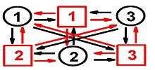
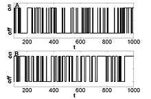
In biophysics and related fields, reduced dimension forms (RDFs) are unique on-off mechanisms for random walks that generate two-state trajectories (see Fig. 1 for an example of a RDF and Fig. 2 for an example of a two-state trajectory). It has been shown that RDFs solve two-state trajectories, since only one RDF can be constructed from the data,[1] where this property does not hold for on-off kinetic schemes, where many kinetic schemes can be constructed from a particular two-state trajectory (even from an ideal on-off trajectory). Two-state time trajectories are very common in measurements in chemistry, physics, and the biophysics of individual molecules [2][3] (e.g. measurements of protein dynamics and DNA and RNA dynamics,[4][5][6][7][8][9][10] activity of ion channels,[11][12][13] enzyme activity,[14][15][16][17][18][19][20][21][22][23][24] quantum dots [25][26][27][28][29][30][31][32]) thus making RDFs an important tool in the analysis of data in these fields.
Since RDFs are uniquely obtained from the data,[33][34] they have many advantages over other mathematical and statistical methods that were developed for solving two-state trajectories.[35][36][37][38][39][40][41][42][43][44][45][46][47]


Description of RDF
A RDF is a lattice of substates, each substate represents either the on state or the off state, and has a particular number (see Figure 1). The connections are only among substates of different states. A simulation of an on-off trajectory from a RDF is made with a generalized Gillespie algorithm, where here a random jumping time is first taken from density functions that are (usually) not exponential using the rejection method, and then the specific next substate is chosen according to the jumping probabilities that are determined from the jumping time probability density functions. A RDF can have irreversible connections, yet, it generates an on-off trajectory that has the property of microscopic reversibility, meaning that the physical system fluctuates around equilibrium.
Two-state trajectories
A two-state trajectory is a fluctuating signal made of on periods and off periods; an on period, and then an off period, and so on (see, Fig. 2). In most cases where this signal appears in applications in science, the trajectory is random; that is, the length of the on and off periods changes, and is a random quantity. There may be correlations in the trajectory; e.g., when we see a short off period and the next on period is relatively long (that is, long with a large probability), we say that there are off-on correlations. In principle, there are 4 independent types of correlations in two-state trajectories: on-on, on-off, off-on, and off-off. Two-state trajectories can be obtained from on-off kinetic schemes, RDFs, or any other stochastic equation of motion (with a clear on-off definition). In experiments from individual molecules, two-state trajectories are common, where from the trajectory we aim at finding the right model of the process.[48]
Using RDFs in solving two-state trajectories
Properties of RDFs in solving two-state trajectories

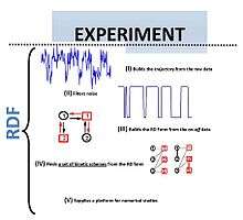
It was shown in Ref. 1[1] that RDFs are unique is the sense that a particular RDF generates a particular time trajectory (in a statistical sense), and a time trajectory is associated with only one RDF. This property does not hold for on-off kinetic schemes, where from a trajectory several kinetic schemes can be constructed ; see for example,.[1] RDFs are also constructed more reliably from the data than kinetic schemes.[33] Figure 3 illustrates RDFs, kinetic schemes and two-state trajectories, and the relations among these. Given a two-state trajectory (generated from any mechanism), it is safer to go from the data and construct a RDF, rather than trying to construct the kinetic scheme from the data directly. With the constructed RDF, one can find several possible kinetic schemes very accurately (usually, one eventually tries constructing a kinetic scheme from the data), where these kinetic schemes are all equivalent (with regard to the data).
The software RDF
- Based on RDFs, software for deducing the correct mechanisms from real data (e.g. two-state trajectories) is designed.[49] See Figure 4 for an illustration of the aims of the software. The software is named RDF.

References
- 1 2 3 O. Flomenbom, and R. J. Silbey, Utilizing the information content in two-state trajectories, Proc. Natl. Acad. Sci. USA 103, 10907-10910 (2006).
- ↑ Moerner, W. E. & Orrit, M. (1999) Science 283, 1670–1676.
- ↑ Weiss, S. (1999) Science 283, 1676–1683.
- ↑ Schuler, B., Lipman, E. A. & Eaton, W. A. (2002) Nature 419, 743–747.
- ↑ Yang, H., Luo, G., Karnchanaphanurach, P., Louie, T., Rech, I., Cova, S., Xun, L., Xie, X. S. (2003) Science 302, 262–266.
- ↑ Min, W., Lou, G., Cherayil, B. J., Kou, S. C., & Xie, X. S. (2005) Phys. Rev. Lett. 94, 198302.
- ↑ Rhoades, E., Gussakovsky, E. & Haran, G. (2003) Proc. Natl. Acad. Sci. USA 100, 3197–3202.
- ↑ Zhuang, X., Kim, H., Pereira, M. J. B., Babcock, H. P., Walter, N. G., & Chu, S. (2002) Science 296, 1473–1476.
- ↑ Barsegov, V. & Thirumalai, D. (2005) Phys. Rev. Lett. 95, 168302-1-4.
- ↑ Kolomeisky, A. B. & Fisher, M. E. (2000) J. Chem. Phys. 113, 10867-10877.
- ↑ Neher, E. & Sakmanm, B. (1976) Nature 260, 799–802.
- ↑ Kasianowicz, J. J., Brandin, E., Branton, D., & Deamer, D. W. (1996) Proc. Natl. Acad. Sci. USA 93, 13770–13773.
- ↑ Kullman, L., Gurnev, P. A., Winterhalter, M., & Bezrukov, S. M. (2006) Phys. Rev. Lett. 96, 038101-038104.
- ↑ Lu, H., Xun, L. & Xie, X. S. (1998) Science 282, 1877–1882.
- ↑ . Edman, L., Földes-Papp, Z., Wennmalm, S. & Rigler, R. (1999) Chem. Phys. 247, 11–22.
- ↑ Velonia, K., Flomenbom, O., Loos, D., Masuo, S., Cotlet, M., Engelborghs, Y., Hofkens, J., Rowan, A. E., Klafter, J., Nolte, R. J. M., et al. (2005) Angew. Chem. Int. Ed. 44, 560–564.
- ↑ Flomenbom, O., Velonia, K., Loos, D., Masuo, S., Cotlet, M., Engelborghs, Y., Hofkens, J., Rowan, A. E., Nolte, R. J. M., Van der Auweraer, M., et al. (2005) Proc. Natl. Acad. Sci. USA. 102, 2368–2372.
- ↑ English, B. P., Min, W., van Oijen, A. M., Lee, K. T., Luo, G., Sun, H., Cherayil, B. J., Kou, S. C., & Xie., X. S. (2006) Nat. chem. Biol. 2, 87–94.
- ↑ Agmon, N. (2000) J. Phys. Chem. B 104, 7830–7834.
- ↑ Qian, H. & Elson, E. L. (2002) Biophys. Chem. 101, 565–576.
- ↑ Kou, S. C., Cherayil, B. J., Min, W., English, B. P., & Xie, X. S. (2005) J. Phys. Chem. B 109, 19068–19081.
- ↑ Sung, J. Y. & Silbey, R. J. (2005) Chem. Phys. Lett. 415, 10–14.
- ↑ Shaevitz, J. W., Block, S. M., & Schnitzer, M. J. (2005) Biophys. J. 89, 2277–2285.
- ↑ Goychuk, I. & Hänggi, P. (2004) Phys. Rev. E 70, 051915-1-9.
- ↑ Nie, S., Chiu, D. T. & Zare R. N. (1994) Science 266, 1018–1021.
- ↑ Shusterman, R., Alon, S., Gavrinyov, T., & Krichevsky, O. (2004) Phys. Rev. Lett. 92, 048303-1-4.
- ↑ Zumofen, G., Hohlbein, J. & Hübner, C. G. (2004) Phys. Rev. Lett. 93, 260601-1-4.
- ↑ Cohen, A. E. & Moerner, W. E. (2006) Proc. Natl. Acad. Sci. USA. 103, 4362–4365.
- ↑ Dickson, R. M., Cubitt, A. B., Tsien, R. Y., & Moerner, W. E. (1997) Nature 388, 355-358.
- ↑ Chung, I. & Bawendi M. G. (2004) Phys. Rev. B. 70, 165304-1-5.
- ↑ Barkai, E., Jung, Y. & Silbey, R. (2004) Annu. Rev. Phys. Chem. 55, 457-507.
- ↑ Tang, J. & Marcus, R. A. (2005) J. Chem. Phys. 123, 204511-1-6.
- 1 2 O. Flomenbom, and R. J. Silbey, Toolbox for analyzing finite two-state trajectories, Phys. Rev. E 78, 066105 (2008).
- ↑ O Flomenbom, Adv. Chem. Phys., in press (2011).
- ↑ Horn, R. & Lange, K. (1983) Biophys. J. 43, 207–223.
- ↑ Qin. F., Auerbach, A. & Sachs, F. (2000) Biophys. J. 79, 1915–1927.
- ↑ Bruno, W. J., Yang, J. & Pearson, J. (2005) Proc. Natl. Acad. Sci. USA. 102, 6326–6331.
- ↑ Bauer, R. J., Bowman, B. F. & Kenyon, J. L. (1987) Biophys. J. 52, 961 – 978.
- ↑ Kienker, P. (1989) Proc. R. Soc. London B. 236, 269–309.
- ↑ Fredkin, D. R. & Rice, J. A. (1986) J. Appl. Prob. 23, 208–214.
- ↑ Colquhoun, D. & Hawkes A. G. (1982) Philos. Trans. R. Soc. Lond. B Biol. Sci. 300, 1–59.
- ↑ Song, L. & Magdeby, K. L. (1994) Biophys. J. 67, 91–104.
- ↑ Cao, J. (2000) Chem. Phys. Lett. 327, 38–44.
- ↑ Vlad, M. O., Moran, F., Schneider, F. W., & Ross, J. (2002) Proc. Natl. Acad. Sci. USA. 99, 12548–12555.
- ↑ Yang, S. & Cao, J. (2002) J. Chem. Phys. 117, 10996–11009.
- ↑ Šanda, F., & Mukamel, S. (2006) J. Chem. Phys. 108, 124103-1-15.
- ↑ Allegrini, P., Aquino, G., Grigolini, P., Palatella, L., & Rosa, A. (2003) Phys. Rev. E 68, 056123-1-11.
- ↑ Flomenbom, O., Klafter, J. & Szabo, A. (2005) Biophys. J. 88, 3780–3783.
- ↑ Please see, http://www.flomenbom.net/codes.html