Nonparametric regression
| Part of a series on Statistics |
| Regression analysis |
|---|
 |
| Models |
| Estimation |
| Background |
|
Nonparametric regression is a category of regression analysis in which the predictor does not take a predetermined form but is constructed according to information derived from the data. Nonparametric regression requires larger sample sizes than regression based on parametric models because the data must supply the model structure as well as the model estimates.
Gaussian process regression or Kriging
In Gaussian process regression, also known as Kriging, a Gaussian prior is assumed for the regression curve. The errors are assumed to have a multivariate normal distribution and the regression curve is estimated by its posterior mode. The Gaussian prior may depend on unknown hyperparameters, which are usually estimated via empirical Bayes.
Smoothing splines have an interpretation as the posterior mode of a Gaussian process regression.
Kernel regression

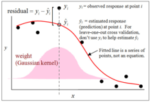
Kernel regression estimates the continuous dependent variable from a limited set of data points by convolving the data points' locations with a kernel function—approximately speaking, the kernel function specifies how to "blur" the influence of the data points so that their values can be used to predict the value for nearby locations.
Nonparametric multiplicative regression


Nonparametric multiplicative regression (NPMR) is a form of nonparametric regression based on multiplicative kernel estimation. Like other regression methods, the goal is to estimate a response (dependent variable) based on one or more predictors (independent variables). NPMR can be a good choice for a regression method if the following are true:
- The shape of the response surface is unknown.
- The predictors are likely to interact in producing the response; in other words, the shape of the response to one predictor is likely to depend on other predictors.
- The response is either a quantitative or binary (0/1) variable.
This is a smoothing technique that can be cross-validated and applied in a predictive way.
- NPMR behaves like an organism
NPMR has been useful for modeling the response of an organism to its environment. Organismal response to environment tends to be nonlinear and have complex interactions among predictors. NPMR allows you to model automatically the complex interactions among predictors in much the same way that organisms integrate the numerous factors affecting their performance.[1]
A key biological feature of an NPMR model is that failure of an organism to tolerate any single dimension of the predictor space results in overall failure of the organism. For example, assume that a plant needs a certain range of moisture in a particular temperature range. If either temperature or moisture fall outside the tolerance of the organism, then the organism dies. If it is too hot, then no amount of moisture can compensate to result in survival of the plant. Mathematically this works with NPMR because the product of the weights for the target point is zero or near zero if any of the weights for individual predictors (moisture or temperature) are zero or near zero. Note further that in this simple example, the second condition listed above is probably true: the response of the plant to moisture probably depends on temperature and vice versa.
Optimizing the selection of predictors and their smoothing parameters in a multiplicative model is computationally intensive. With a large pool of predictors, the computer must search through a huge number of potential models in search for the best model. The best model has the best fit, subject to overfitting constraints or penalties (see below).[2][3]
- The local model
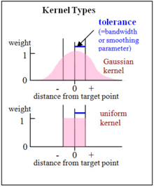
NPMR can be applied with several different kinds of local models. By "local model" we mean the way that data points near a target point in the predictor space are combined to produce an estimate for the target point. The most common choices for the local models are the local mean estimator, a local linear estimator, or a local logistic estimator. In each case the weights can be extended multiplicatively to multiple dimensions.
In words, the estimate of the response is a local estimate (for example a local mean) of the observed values, each value weighted by its proximity to the target point in the predictor space, the weights being the product of weights for individual predictors. The model allows interactions, because weights for individual predictors are combined by multiplication rather than addition.
- Overfitting controls
Understanding and using these controls on overfitting is essential to effective modeling with nonparametric regression. Nonparametric regression models can become overfit either by including too many predictors or by using small smoothing parameters (also known as bandwidth or tolerance). This can make a big difference with special problems, such as small data sets or clumped distributions along predictor variables.
The methods for controlling overfitting differ between NPMR and the generalized linear modeling (GLMs). The most popular overfitting controls for GLMs are the Akaike information criterion (AIC) and the Bayesian information criterion (BIC) for model selection. The AIC and BIC depend on the number of parameters in a model. Because NPMR models do not have explicit parameters as such, these are not directly applicable to NPMR models. Instead, one can control overfitting by setting a minimum average neighborhood size, minimum data:predictor ratio, and a minimum improvement required to add a predictor to a model.
Nonparametric regression models sometimes use an AIC based on the "effective number of parameters".[4] This penalizes a measure of fit by the trace of the smoothing matrix—essentially how much each data point contributes to estimating itself, summed across all data points. If, however, you use leave-one-out cross validation in the model fitting phase, the trace of the smoothing matrix is always zero, corresponding to zero parameters for the AIC. Thus, NPMR with cross-validation in the model fitting phase already penalizes the measure of fit, such that the error rate of the training data set is expected to approximate the error rate in a validation data set. In other words, the training error rate approximates the prediction (extra-sample) error rate.
- Related techniques
NPMR is essentially a smoothing technique that can be cross-validated and applied in a predictive way. Many other smoothing techniques are well known, for example smoothing splines and wavelets. The optimal choice of a smoothing method depends on the specific application. Nonparametric regression models always fits for larger data
Regression trees
Decision tree learning algorithms can be applied to learn to predict a dependent variable from data.[5] Although the original CART formulation applied only to predicting univariate data, the framework can be used to predict multivariate data including time series.[6]
See also
- Local regression
- Non-parametric statistics
- Semiparametric regression
- Isotonic regression
- Multivariate adaptive regression splines
References
- ↑ McCune, B. (2006). "Non-parametric habitat models with automatic interactions". Journal of Vegetation Science. 17 (6): 819–830. doi:10.1658/1100-9233(2006)17[819:NHMWAI]2.0.CO;2.
- ↑ Grundel, R.; Pavlovic, N. B. (2007). "Response of bird species densities to habitat structure and fire history along a Midwestern open–forest Gradient". The Condor. 109 (4): 734–749. doi:10.1650/0010-5422(2007)109[734:ROBSDT]2.0.CO;2.
- ↑ DeBano, S. J.; Hamm, P. B.; Jensen, A.; Rondon, S. I.; Landolt, P. J. (2010). "Spatial and temporal dynamics of potato tuberworm (Lepidoptera: Gelechiidae) in the Columbia Basin of the Pacific Northwest". Environmental Entomology. 39 (1): 1–14. doi:10.1603/EN08270.
- ↑ Hastie, T.; Tibsharani, R.; Friedman, J. (2001). The Elements of Statistical Learning. New York: Springer. p. 205. ISBN 0387952845.
- ↑ Breiman, Leo; Friedman, J. H.; Olshen, R. A.; Stone, C. J. (1984). Classification and regression trees. Monterey, CA: Wadsworth & Brooks/Cole Advanced Books & Software. ISBN 978-0-412-04841-8.
- ↑ Segal, M.R. (1992). "Tree-structured methods for longitudinal data". Journal of the American Statistical Association. 87 (418): 407–418. JSTOR 2290271. doi:10.2307/2290271.
Further reading
- Bowman, A. W.; Azzalini, A. (1997). Applied Smoothing Techniques for Data Analysis. Oxford: Clarendon Press. ISBN 0-19-852396-3.
- Fan, J.; Gijbels, I. (1996). Local Polynomial Modelling and its Applications. Boca Raton: Chapman and Hall. ISBN 0-412-98321-4.
- Henderson, D. J.; Parmeter, C. F. (2015). Applied Nonparametric Econometrics. New York: Cambridge University Press. ISBN 978-1-107-01025-3.
- Li, Q.; Racine, J. (2007). Nonparametric Econometrics: Theory and Practice. Princeton: Princeton University Press. ISBN 978-0-691-12161-1.
- Pagan, A.; Ullah, A. (1999). Nonparametric Econometrics. New York: Cambridge University Press. ISBN 0-521-35564-8.
External links
- HyperNiche, software for nonparametric multiplicative regression.
- Scale-adaptive nonparametric regression (with Matlab software).