Tree rearrangement
Tree rearrangements are used in heuristic algorithms devoted to searching for an optimal tree structure. They can be applied to any set of data that are naturally arranged into a tree, but have most applications in computational phylogenetics, especially in maximum parsimony and maximum likelihood searches of phylogenetic trees, which seek to identify one among many possible trees that best explains the evolutionary history of a particular gene or species.
Basic tree rearrangements
 Nearest neighbor interchange (NNI)
 Subtree pruning and regrafting (SPR)
 Tree bisection and reconnection (TBR)
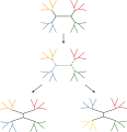
The simplest tree-rearrangement, known as nearest-neighbor interchange, exchanges the connectivity of four subtrees within the main tree. Because there are three possible ways of connecting four subtrees,[1] and one is the original connectivity, each interchange creates two new trees. Exhaustively searching the possible nearest-neighbors for each possible set of subtrees is the slowest but most optimizing way of performing this search. An alternative, more wide-ranging search, subtree pruning and regrafting (SPR), selects and removes a subtree from the main tree and reinserts it elsewhere on the main tree to create a new node. Finally, tree bisection and reconnection (TBR) detaches a subtree from the main tree at an interior node and then attempts all possible connections between edges of the two trees thus created. The increasing complexity of the tree rearrangement technique correlates with increasing computational time required for the search, although not necessarily with their performance.[2]
SPR can be further divided into uSPR: Unrooted SPR, rSPR: Rooted SPR. uSPR is applied to unrooted trees, and goes like this: break any edge. Join one end of the edge (selected arbitrarily) to any other edge in the tree. rSPR is applied to rooted trees*, and goes: break any edge except the edge leading to the root node. Join one end of the edge (specifically: the end of the edge that is FURTHEST from the root) and attach it to any other edge of the tree.[3]
* In this example the root of the tree is marked by a node of degree one, meaning that all nodes in the tree have either degree 1 or degree 3. An alternative approach, used in Bordewich and Semple, is to consider the root node to have degree 2, and to have a special rule for rSPR.
The number of SPR[4] or TBR[5] moves needed to get from one tree to another can be calculated by producing a Maximum Agreement Forest comprising (respectively) rooted or unrooted trees. This problem is NP hard but Fixed Parameter Tractable.
Tree fusion
The simplest type of tree fusion begins with two trees already identified as near-optimal; thus, they most likely have the majority of their nodes correct but may fail to resolve individual tree "leaves" properly; for example, the separation ((A,B),(C,D)) at a branch tip versus ((A,C),(B,D)) may be unresolved.[1] Tree fusion swaps these two solutions between two otherwise near-optimal trees. Variants of the method use standard genetic algorithms with a defined objective function to swap high-scoring subtrees into main trees that are high-scoring overall.[6]
Sectorial search
An alternative strategy is to detach part of the tree (which can be selected at random, or using a more strategic approach) and to perform TBR/SPR/NNI on this sub-tree. This optimized sub-tree can then be replaced on the main tree, hopefully improving the p-score.[7]
Tree drifting
To avoid entrapment in local optima, a 'simulated annealing' approach can be used, whereby the algorithm is occasionally permitted to entertain sub-optimal candidate trees, with a probability related to how far they are from the optimum.[7]
Tree fusing
Once a range of equally-optimal trees have been gathered, it is often possible to find a better tree by combining the "good bits" of separate trees. Sub-groups with an identical composition but different topology can be switched and the resultant trees evaluated.[7]
References
- 1 2 Felsenstein J. (2004). Inferring Phylogenies Sinauer Associates: Sunderland, MA.
- ↑ Takahashi K, Nei M. (2000). Efficiencies of fast algorithms of phylogenetic inference under the criteria of maximum parsimony, minimum evolution, and maximum likelihood when a large number of sequences are used. Mol Biol Evol 17(8):1251-8.
- ↑ Bordewich M, Semple C. 2005. On the computational complexity of the rooted subtree prune and regraft distance Ann. Comb. 8:409–23
- ↑ WHIDDEN, C., BEIKO, R. G. and ZEH, N. 2016. Fixed-Parameter and Approximation Algorithms for Maximum Agreement Forests of Multifurcating Trees. Algorithmica, 74, 1019–1054
- ↑ CHEN, J., FAN, J.-H. and SZE, S.-H. 2015. Parameterized and approximation algorithms for maximum agreement forest in multifurcating trees. Theoretical Computer Science, 562, 496–512.
- ↑ Matsuda H. (1996). Protein phylogenetic inference using maximum likelihood with a genetic algorithm. Pacific Symposium on Biocomputing 1996, pp512-23.
- 1 2 3 Goloboff, P. (1999). Analyzing Large Data Sets in Reasonable Times: Solutions for Composite Optima. Cladistics, 15(4), 415–428. doi:10.1006/clad.1999.0122