Lorenz system

The Lorenz system is a system of ordinary differential equations first studied by Edward Lorenz. It is notable for having chaotic solutions for certain parameter values and initial conditions. In particular, the Lorenz attractor is a set of chaotic solutions of the Lorenz system which, when plotted, resemble a butterfly or figure eight.
Overview
In 1963, Edward Lorenz developed a simplified mathematical model for atmospheric convection.[1] The model is a system of three ordinary differential equations now known as the Lorenz equations:

Here , , and make up the system state, is time, and , , are the system parameters. The Lorenz equations also arise in simplified models for lasers,[2] dynamos,[3] thermosyphons,[4] brushless DC motors,[5] electric circuits,[6] chemical reactions[7] and forward osmosis.[8]


From a technical standpoint, the Lorenz system is nonlinear, non-periodic, three-dimensional and deterministic. The Lorenz equations have been the subject of hundreds of research articles, and at least one book-length study.[9]
Analysis
One normally assumes that the parameters , , and are positive. Lorenz used the values , and . The system exhibits chaotic behavior for these (and nearby) values.[10]


If then there is only one equilibrium point, which is at the origin. This point corresponds to no convection. All orbits converge to the origin, which is a global attractor, when .[11]

A pitchfork bifurcation occurs at , and for two additional critical points appear at: and These correspond to steady convection. This pair of equilibrium points is stable only if


which can hold only for positive if . At the critical value, both equilibrium points lose stability through a Hopf bifurcation.[12]

When , , and , the Lorenz system has chaotic solutions (but not all solutions are chaotic). Almost all initial points will tend to an invariant set – the Lorenz attractor – a strange attractor and a fractal. Its Hausdorff dimension is estimated to be 2.06 ± 0.01, and the correlation dimension is estimated to be 2.05 ± 0.01.[13] The exact Lyapunov dimension (Kaplan-Yorke dimension) formula of the global attractor can be found analytically under classical restrictions on the parameters
- [14]
- .

The Lorenz attractor is difficult to analyze, but the action of the differential equation on the attractor is described by a fairly simple geometric model.[15] Proving that this is indeed the case is the fourteenth problem on the list of Smale's problems. This problem was the first one to be resolved, by Warwick Tucker in 2002.[16]
For other values of , the system displays knotted periodic orbits. For example, with it becomes a T(3,2) torus knot.

| Example solutions of the Lorenz system for different values of ρ | |
|---|---|
 |
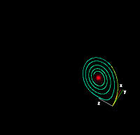 |
| ρ=14, σ=10, β=8/3 (Enlarge) | ρ=13, σ=10, β=8/3 (Enlarge) |
 |
 |
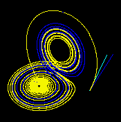
| ρ=15, σ=10, β=8/3 (Enlarge) | ρ=28, σ=10, β=8/3 (Enlarge) |
| For small values of ρ, the system is stable and evolves to one of two fixed point attractors. When ρ is larger than 24.74, the fixed points become repulsors and the trajectory is repelled by them in a very complex way. | |
| Java animation showing evolution for different values of ρ | |
| Sensitive dependence on the initial condition | ||
|---|---|---|
| Time t=1 (Enlarge) | Time t=2 (Enlarge) | Time t=3 (Enlarge) |
 |
 |
 |
| These figures — made using ρ=28, σ = 10 and β = 8/3 — show three time segments of the 3-D evolution of 2 trajectories (one in blue, the other in yellow) in the Lorenz attractor starting at two initial points that differ only by 10−5 in the x-coordinate. Initially, the two trajectories seem coincident (only the yellow one can be seen, as it is drawn over the blue one) but, after some time, the divergence is obvious. | ||
| Java animation of the Lorenz attractor shows the continuous evolution. | ||
MATLAB simulation
% Solve over time interval [0,100] with initial conditions [1,1,1]
% 'f' is set of differential equations
% 'a' is array containing x, y, and z variables
% 't' is time variable

sigma = 10;
beta = 8/3;
rho = 28;
f = @(t,a) [-sigma*a(1) + sigma*a(2); rho*a(1) - a(2) - a(1)*a(3); -beta*a(3) + a(1)*a(2)];
[t,a] = ode45(f,[0 100],[1 1 1]);     % Runge-Kutta 4th/5th order ODE solver
plot3(a(:,1),a(:,2),a(:,3))
Mathematica simulation
a = 10; b = 8/3; r = 28;
x = 1; y = 1; z = 1;points = {{1,1,1}};
i := AppendTo[points, {x = N[x + (a*y - a*x)/100], y = N[y + (-x*z + r*x - y)/100], z = N[z + (x*y - b*z)/100]}]

Do[i, {3000}]
ListPointPlot3D[points, PlotStyle -> {Red, PointSize[Tiny]}]
fancier way:
tend = 50;
eq = {x'[t] == σ (y[t] - x[t]),
      y'[t] == x[t] (ρ - z[t]) - y[t],
      z'[t] == x[t] y[t] - β z[t]};
init = {x[0] == 10, y[0] == 10, z[0] == 10};
pars = {σ→10, ρ→28, β→8/3};
{xs, ys, zs} =
  NDSolveValue[{eq /. pars, init}, {x, y, z}, {t, 0, tend}];
ParametricPlot3D[{xs[t], ys[t], zs[t]}, {t, 0, tend}]
Python simulation
import numpy as np
import matplotlib.pyplot as plt
from scipy.integrate import odeint
from mpl_toolkits.mplot3d import Axes3D

rho = 28.0
sigma = 10.0
beta = 8.0 / 3.0

def f(state, t):
  x, y, z = state  # unpack the state vector
  return sigma * (y - x), x * (rho - z) - y, x * y - beta * z  # derivatives

state0 = [1.0, 1.0, 1.0]
t = np.arange(0.0, 40.0, 0.01)

states = odeint(f, state0, t)

fig = plt.figure()
ax = fig.gca(projection='3d')
ax.plot(states[:,0], states[:,1], states[:,2])
plt.show()
Derivation of the Lorenz equations as a model of atmospheric convection
The Lorenz equations are derived from the Oberbeck-Boussinesq approximation to the equations describing fluid circulation in a shallow layer of fluid, heated uniformly from below and cooled uniformly from above.[1] This fluid circulation is known as Rayleigh-Bénard convection. The fluid is assumed to circulate in two dimensions (vertical and horizontal) with periodic rectangular boundary conditions.
The partial differential equations modeling the system's stream function and temperature are subjected to a spectral Galerkin approximation: the hydrodynamic fields are expanded in Fourier series, which are then severely truncated to a single term for the stream function and two terms for the temperature. This reduces the model equations to a set of three coupled, nonlinear ordinary differential equations. A detailed derivation may be found, for example, in nonlinear dynamics texts.[17] The Lorenz system is a reduced version of a larger system studied earlier by Barry Saltzman.[18]
Gallery
 A solution in the Lorenz attractor plotted at high resolution in the x-z plane.
 A solution in the Lorenz attractor rendered as an SVG.
- An animation showing trajectories of multiple solutions in a Lorenz system.
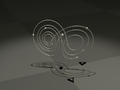 A solution in the Lorenz attractor rendered as a metal wire to show direction and 3D structure.
- An animation showing the divergence of nearby solutions to the Lorenz system.
 A visualization of the Lorenz attractor near an intermittent cycle.
See also
Notes
- 1 2 Lorenz (1963)
- ↑ Haken (1975)
- ↑ Knobloch (1981)
- ↑ Gorman, Widmann & Robbins (1986)
- ↑ Hemati (1994)
- ↑ Cuomo & Oppenheim (1993)
- ↑ Poland (1993)
- ↑ Tzenov (2014)
- ↑ Sparrow (1982)
- ↑ Hirsch, Smale & Devaney (2003), pp. 303–305
- ↑ Hirsch, Smale & Devaney (2003), pp. 306+307
- ↑ Hirsch, Smale & Devaney (2003), pp. 307+308
- ↑ Grassberger & Procaccia (1983)
- ↑ Leonov et al. (2016)
- ↑ Guckenheimer, John; Williams, R. F. (1979-12-01). "Structural stability of Lorenz attractors". Publications Mathématiques de l'Institut des Hautes Études Scientifiques. 50 (1): 59–72. ISSN 0073-8301. doi:10.1007/BF02684769.
- ↑ Tucker (2002)
- ↑ Hilborn (2000), Appendix C; Bergé, Pomeau & Vidal (1984), Appendix D
- ↑ Saltzman (1962)
References
- Bergé, Pierre; Pomeau, Yves; Vidal, Christian (1984). Order within Chaos: Towards a Deterministic Approach to Turbulence. New York: John Wiley & Sons. ISBN 978-0-471-84967-4.
- Cuomo, Kevin M.; Oppenheim, Alan V. (1993). "Circuit implementation of synchronized chaos with applications to communications". Physical Review Letters. 71 (1): 65–68. Bibcode:1993PhRvL..71...65C. ISSN 0031-9007. PMID 10054374. doi:10.1103/PhysRevLett.71.65.
- Gorman, M.; Widmann, P.J.; Robbins, K.A. (1986). "Nonlinear dynamics of a convection loop: A quantitative comparison of experiment with theory". Physica D. 19 (2): 255–267. Bibcode:1986PhyD...19..255G. doi:10.1016/0167-2789(86)90022-9.
- Grassberger, P.; Procaccia, I. (1983). "Measuring the strangeness of strange attractors". Physica D. 9 (1–2): 189–208. Bibcode:1983PhyD....9..189G. doi:10.1016/0167-2789(83)90298-1.
- Haken, H. (1975). "Analogy between higher instabilities in fluids and lasers". Physics Letters A. 53 (1): 77–78. Bibcode:1975PhLA...53...77H. doi:10.1016/0375-9601(75)90353-9.
- Hemati, N. (1994). "Strange attractors in brushless DC motors". IEEE Transactions on Circuits and Systems I: Fundamental Theory and Applications. 41 (1): 40–45. ISSN 1057-7122. doi:10.1109/81.260218.
- Hilborn, Robert C. (2000). Chaos and Nonlinear Dynamics: An Introduction for Scientists and Engineers (second ed.). Oxford University Press. ISBN 978-0-19-850723-9.
- Hirsch, Morris W.; Smale, Stephen; Devaney, Robert (2003). Differential Equations, Dynamical Systems, & An Introduction to Chaos (Second ed.). Boston, MA: Academic Press. ISBN 978-0-12-349703-1.
- Lorenz, Edward Norton (1963). "Deterministic nonperiodic flow". Journal of the Atmospheric Sciences. 20 (2): 130–141. Bibcode:1963JAtS...20..130L. doi:10.1175/1520-0469(1963)020<0130:DNF>2.0.CO;2.
- Knobloch, Edgar (1981). "Chaos in the segmented disc dynamo". Physics Letters A. 82 (9): 439–440. Bibcode:1981PhLA...82..439K. doi:10.1016/0375-9601(81)90274-7.
- Pchelintsev, A.N. (2014). "Numerical and Physical Modeling of the Dynamics of the Lorenz System". Numerical Analysis and Applications. 7 (2): 159–167. doi:10.1134/S1995423914020098.
- Poland, Douglas (1993). "Cooperative catalysis and chemical chaos: a chemical model for the Lorenz equations". Physica D. 65 (1): 86–99. Bibcode:1993PhyD...65...86P. doi:10.1016/0167-2789(93)90006-M.
- Tzenov, Stephan (2014). "Strange Attractors Characterizing the Osmotic Instability". arXiv:1406.0979v1
 [physics.flu-dyn].
 - Saltzman, Barry (1962). "Finite Amplitude Free Convection as an Initial Value Problem—I". Journal of the Atmospheric Sciences. 19 (4): 329–341. Bibcode:1962JAtS...19..329S. doi:10.1175/1520-0469(1962)019<0329:FAFCAA>2.0.CO;2.
- Sparrow, Colin (1982). The Lorenz Equations: Bifurcations, Chaos, and Strange Attractors. Springer.
- Tucker, Warwick (2002). "A Rigorous ODE Solver and Smale's 14th Problem" (PDF). Foundations of Computational Mathematics. 2 (1): 53–117. doi:10.1007/s002080010018.
- Leonov, G.A.; Kuznetsov, N.V.; Korzhemanova, N.A.; Kusakin, D.V. (2016). "Lyapunov dimension formula for the global attractor of the Lorenz system". Communications in Nonlinear Science and Numerical Simulation. 41: 84–103. doi:10.1016/j.cnsns.2016.04.032.
Further reading
- G.A. Leonov & N.V. Kuznetsov (2015). "On differences and similarities in the analysis of Lorenz, Chen, and Lu systems" (PDF). Applied Mathematics and Computation. 256: 334–343. doi:10.1016/j.amc.2014.12.132.
External links
| Wikimedia Commons has media related to Lorenz attractors. |
- Hazewinkel, Michiel, ed. (2001) [1994], "Lorenz attractor", Encyclopedia of Mathematics, Springer Science+Business Media B.V. / Kluwer Academic Publishers, ISBN 978-1-55608-010-4
- Weisstein, Eric W. "Lorenz attractor". MathWorld.
- Lorenz attractor by Rob Morris, Wolfram Demonstrations Project.
- Lorenz equation on planetmath.org
- Synchronized Chaos and Private Communications, with Kevin Cuomo. The implementation of Lorenz attractor in an electronic circuit.
- Lorenz attractor interactive animation (you need the Adobe Shockwave plugin)
- 3D Attractors: Mac program to visualize and explore the Lorenz attractor in 3 dimensions
- Lorenz Attractor implemented in analog electronic
- Lorenz Attractor interactive animation (implemented in Ada with GTK+. Sources & executable)
- Web based Lorenz Attractor (implemented in javascript / html /css)

