Kruskal's algorithm
 | |
| Class | Minimum spanning tree |
|---|---|
| Data structure | Disjoint-set data structure |
| Average performance | |
| Worst-case space complexity | |
| Graph and tree search algorithms |
|---|
| Listings |
|
| Related topics |
Kruskal's algorithm is a minimum-spanning-tree algorithm which finds an edge of the least possible weight that connects any two trees in the forest.[1] It is a greedy algorithm in graph theory as it finds a minimum spanning tree for a connected weighted graph adding increasing cost arcs at each step.[1] This means it finds a subset of the edges that forms a tree that includes every vertex, where the total weight of all the edges in the tree is minimized. If the graph is not connected, then it finds a minimum spanning forest (a minimum spanning tree for each connected component).
This algorithm first appeared in Proceedings of the American Mathematical Society, pp. 48–50 in 1956, and was written by Joseph Kruskal.[2]
Other algorithms for this problem include Prim's algorithm, Reverse-delete algorithm, and Borůvka's algorithm.
Algorithm
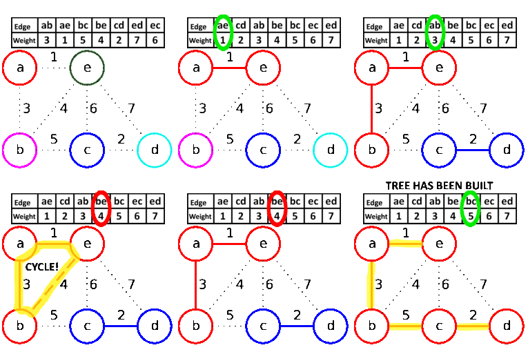
- create a forest F (a set of trees), where each vertex in the graph is a separate tree
- create a set S containing all the edges in the graph
- while S is nonempty and F is not yet spanning
- remove an edge with minimum weight from S
- if the removed edge connects two different trees then add it to the forest F, combining two trees into a single tree
At the termination of the algorithm, the forest forms a minimum spanning forest of the graph. If the graph is connected, the forest has a single component and forms a minimum spanning tree
Pseudocode
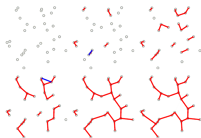
The following code is implemented with disjoint-set data structure:
KRUSKAL(G):
1 A = ∅
2 foreach v ∈ G.V:
3    MAKE-SET(v)
4 foreach (u, v) in G.E ordered by weight(u, v), increasing:
5    if FIND-SET(u) ≠ FIND-SET(v):
6       A = A ∪ {(u, v)}
7       UNION(u, v)
8 return A
Complexity
Kruskal's algorithm can be shown to run in O(E log E) time, or equivalently, O(E log V) time, where E is the number of edges in the graph and V is the number of vertices, all with simple data structures. These running times are equivalent because:
- E is at most V2 and is O(log V).
- Each isolated vertex is a separate component of the minimum spanning forest. If we ignore isolated vertices we obtain V ≤ 2E, so log V is O(log E).
We can achieve this bound as follows: first sort the edges by weight using a comparison sort in O(E log E) time; this allows the step "remove an edge with minimum weight from S" to operate in constant time. Next, we use a disjoint-set data structure (Union&Find) to keep track of which vertices are in which components. We need to perform O(V) operations, as in each iteration we connect a vertex to the spanning tree, two 'find' operations and possibly one union for each edge. Even a simple disjoint-set data structure such as disjoint-set forests with union by rank can perform O(V) operations in O(V log V) time. Thus the total time is O(E log E) = O(E log V).
Provided that the edges are either already sorted or can be sorted in linear time (for example with counting sort or radix sort), the algorithm can use a more sophisticated disjoint-set data structure to run in O(E α(V)) time, where α is the extremely slowly growing inverse of the single-valued Ackermann function.
Example
| Image | Description |
|---|---|
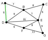 |
AD and CE are the shortest edges, with length 5, and AD has been arbitrarily chosen, so it is highlighted. |
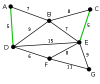 |
CE is now the shortest edge that does not form a cycle, with length 5, so it is highlighted as the second edge. |
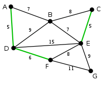 |
The next edge, DF with length 6, is highlighted using much the same method. |
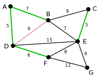 |
The next-shortest edges are AB and BE, both with length 7. AB is chosen arbitrarily, and is highlighted. The edge BD has been highlighted in red, because there already exists a path (in green) between B and D, so it would form a cycle (ABD) if it were chosen. |
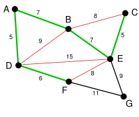 |
The process continues to highlight the next-smallest edge, BE with length 7. Many more edges are highlighted in red at this stage: BC because it would form the loop BCE, DE because it would form the loop DEBA, and FE because it would form FEBAD. |
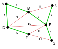 |
Finally, the process finishes with the edge EG of length 9, and the minimum spanning tree is found. |
Proof of correctness
The proof consists of two parts. First, it is proved that the algorithm produces a spanning tree. Second, it is proved that the constructed spanning tree is of minimal weight.
Spanning tree
Let be a connected, weighted graph and let be the subgraph of produced by the algorithm. cannot have a cycle, being within one subtree and not between two different trees. cannot be disconnected, since the first encountered edge that joins two components of would have been added by the algorithm. Thus, is a spanning tree of .
Minimality
We show that the following proposition P is true by induction: If F is the set of edges chosen at any stage of the algorithm, then there is some minimum spanning tree that contains F.
- Clearly P is true at the beginning, when F is empty: any minimum spanning tree will do, and there exists one because a weighted connected graph always has a minimum spanning tree.
- Now assume P is true for some non-final edge set F and let T be a minimum spanning tree that contains F. If the next chosen edge e is also in T, then P is true for F + e. Otherwise, T + e has a cycle C and there is another edge f that is in C but not F. (If there were no such edge f, then e could not have been added to F, since doing so would have created the cycle C.) Then T − f + e is a tree, and it has the same weight as T, since T has minimum weight and the weight of f cannot be less than the weight of e, otherwise the algorithm would have chosen f instead of e. So T − f + e is a minimum spanning tree containing F + e and again P holds.
- Therefore, by the principle of induction, P holds when F has become a spanning tree, which is only possible if F is a minimum spanning tree itself.
See also
- Dijkstra's algorithm
- Prim's algorithm
- Borůvka's algorithm
- Reverse-delete algorithm
- Single-linkage clustering
References
- 1 2 Cormen, Thomas; Charles E Leiserson, Ronald L Rivest, Clifford Stein (2009). Introduction To Algorithms (Third ed.). MIT Press. p. 631. ISBN 0262258102.
- ↑ Kruskal, J. B. (1956). "On the shortest spanning subtree of a graph and the traveling salesman problem". Proceedings of the American Mathematical Society. 7: 48–50. JSTOR 2033241. doi:10.1090/S0002-9939-1956-0078686-7.
- Thomas H. Cormen, Charles E. Leiserson, Ronald L. Rivest, and Clifford Stein. Introduction to Algorithms, Second Edition. MIT Press and McGraw-Hill, 2001. ISBN 0-262-03293-7. Section 23.2: The algorithms of Kruskal and Prim, pp. 567–574.
- Michael T. Goodrich and Roberto Tamassia. Data Structures and Algorithms in Java, Fourth Edition. John Wiley & Sons, Inc., 2006. ISBN 0-471-73884-0. Section 13.7.1: Kruskal's Algorithm, pp. 632..