''k''-medoids

The k-medoids algorithm is a clustering algorithm related to the k-means algorithm and the medoidshift algorithm. Both the k-means and k-medoids algorithms are partitional (breaking the dataset up into groups) and both attempt to minimize the distance between points labeled to be in a cluster and a point designated as the center of that cluster. In contrast to the k-means algorithm, k-medoids chooses datapoints as centers (medoids or exemplars) and works with a generalization of the Manhattan Norm to define distance between datapoints instead of . This method was proposed in 1987^[1] for the work with norm and other distances.

k-medoid is a classical partitioning technique of clustering that clusters the data set of n objects into k clusters known a priori. A useful tool for determining k is the silhouette.

It is more robust to noise and outliers as compared to k-means because it minimizes a sum of pairwise dissimilarities instead of a sum of squared Euclidean distances.

A medoid can be defined as the object of a cluster whose average dissimilarity to all the objects in the cluster is minimal. i.e. it is a most centrally located point in the cluster.

Algorithms

The most common realisation of k-medoid clustering is the Partitioning Around Medoids (PAM) algorithm. PAM uses a greedy search which may not find the optimum solution, but it is faster than exhaustive search . It works as follows:

1. Initialize: select k of the n data points as the medoids
2. Associate each data point to the closest medoid.
3. While the cost of the configuration decreases:
   1. For each medoid m, for each non-medoid data point o:
      1. Swap m and o, recompute the cost (sum of distances of points to their medoid)
      2. If the total cost of the configuration increased in the previous step, undo the swap

Algorithms other than PAM have also been suggested in the literature, including the following Voronoi iteration method: ^{[2] [3]}

1. Select initial medoids
2. Iterate while the cost decreases:
   1. In each cluster, make the point that minimizes the sum of distances within the cluster the medoid
   2. Reassign each point to the cluster defined by the closest medoid determined in the previous step.

Demonstration of PAM

Cluster the following data set of ten objects into two clusters i.e. k = 2.

Consider a data set of ten objects as follows :

Figure 1.1 – distribution of the data

Step 1

Figure 1.2 – clusters after step 1

Randomly are two observations ( and ) are selected as medoids (cluster centers). Manhattan distances are calculated to each center to associate each data object to its nearest medoid (marked in bold).

Data object		Distance to
1	(2, 6)	3	7
2	(3, 4)	0	4
3	(3, 8)	4	8
4	(4, 7)	4	6
5	(6, 2)	5	3
6	(6, 4)	3	1
7	(7, 3)	5	1
8	(7, 4)	4	0
9	(8, 5)	6	2
10	(7, 6)	6	2
Cost		11	9

Since the points (2,6) (3,8) and (4,7) are closer to c₁ hence they form one cluster whilst remaining points form another cluster. Therefore the clusters become:

Cluster₁ = {(3,4)(2,6)(3,8)(4,7)}

Cluster₂ = {(7,4)(6,2)(6,4)(7,3)(8,5)(7,6)}

The total cost of this clustering is the sum of the distance between a data point and its cluster center:

Step 2

Figure 1.3 – clusters after step 2

Select one of the nonmedoids O′

Let us assume O′ = (7,3), i.e. x₇.

So now the medoids are c₁(3,4) and O′(7,3)

If c1 and O′ are new medoids, calculate the total cost involved

By using the formula in the step 1

Figure 2. K-medoids versus k-means. Figs 2.1a-2.1f present a typical example of the k-means convergence to a local minimum. This result of k-means clustering contradicts the obvious cluster structure of data set. In this example, k-medoids algorithm (Figs 2.2a-2.2h) with the same initial position of medoids (Fig. 2.2a) converges to the obvious cluster structure. The small circles are data points, the four ray stars are centroids (means), the nine ray stars are medoids.^[4]

So cost of swapping medoid from c₂ to O′ is

So moving to O′ would be a bad idea, so the previous choice was good. So we try other nonmedoids and found that our first choice was the best. So the configuration does not change and algorithm terminates here (i.e. there is no change in the medoids).

It may happen some data points may shift from one cluster to another cluster depending upon their closeness to medoid.

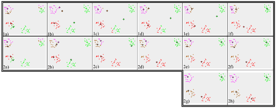
In some standard situations, k-medoids demonstrate better performance than k-means. An example is presented in Fig. 2. The most time-consuming part of the k-medoids algorithm is the calculation of the distances between objects. If a quadratic preprocessing and storage is applicable, the distances matrix can be precomputed to achieve consequent speed-up. See for example,^[3] where the authors also introduce a heuristic to choose the initial k medoids.

Software

• ELKI includes several k-means variants, including an EM-based k-medoids and the original PAM algorithm.
• Julia contains a k-medoid implementation in the JuliaStats clustering package.
• KNIME includes a k-medoid implementation supporting a variety of efficient matrix distance measures, as well as a number of native (and integrated third-party) k-means implementations
• R includes variants of k-means in the "flexclust" package and PAM is implemented in the "cluster" package.
• RapidMiner has an operator named KMedoids, but it does not implement the KMedoids algorithm correctly. Instead, it is a k-means variant, that substitutes the mean with the closest data point (which is not the medoid).
• MATLAB implements PAM, CLARA, and two other algorithms to solve the k-medoid clustering problem.
• Python has an implementation in scikit-learn

References

- ↑ Kaufman, L. and Rousseeuw, P.J. (1987), Clustering by means of Medoids, in Statistical Data Analysis Based on the –Norm and Related Methods, edited by Y. Dodge, North-Holland, 405–416.
- ↑ T. Hastie, R. Tibshirani, and J. Friedman. The Elements of Statistical Learning, Springer (2001), 468–469.
- 1 2 H.S. Park , C.H. Jun, A simple and fast algorithm for K-medoids clustering, Expert Systems with Applications, 36, (2) (2009), 3336–3341.
- ↑ The illustration was prepared with the Java applet, E.M. Mirkes, K-means and K-medoids: applet. University of Leicester, 2011.