Case–Shiller index


The Standard & Poor's Case–Shiller Home Price Indices are repeat-sales house price indices for the United States. There are multiple Case–Shiller home price indices: A national home price index, a 20-city composite index, a 10-city composite index, and twenty individual metro area indices. These indices are calculated and kept monthly by Standard & Poor's, with data points calculated for the time period of January 1987 through the present. The indices kept by Standard and Poor are normalized to have a value of 100 in January 2000. These Indices are based on original work by economists Karl Case and Robert Shiller, in which their team calculated the home price index back to 1890. That index is normalized to have 1890 have a value of 100. The Case–Shiller Index being kept on Shiller's website (http://www.econ.yale.edu/~shiller/data.htm) is updated quarterly. Due to the different set reference points, and perhaps calculation differences, the index numbers provided in each data set can be very different. For example, in 4th quarter 2013, the Standard and Poor 20 city index point was in the 160's, while the index point for 4th quarter on the Shiller data was in the 130's. Shiller claims in his book Irrational Exuberance that such a long series of home prices does not appear to have been published for any country.[1]
History and methodology
The indices are calculated from data on repeat sales of single-family homes, an approach developed by economists Case, Shiller and Allan Weiss who served as the CEO from the company's inception to the Fiserv sale.[2] Case developed a method for comparing repeat sales of the same homes in an effort to study home pricing trends.[2] He was using data from house sales in Boston in the early 1980s, which was going through a housing price boom. While Case argued that such a boom was ultimately unsustainable, he had not considered it a bubble, a commonly used term to describe similar market trends.[2] Case sat down with Shiller, who was researching behavioral finance and economic bubbles, and together formed a repeat-sales index using home sales prices data from other cities across the country.[2] In 1991, while Weiss was in graduate school he formed an informal working relationship with Shiller. Weiss proposed to Case and Shiller to form a company, Case Shiller Weiss, to produce the index periodically with the intent of selling the information to the markets. Fiserv, an information management company, bought Case Shiller Weiss in 2002 and, together with Standard & Poor's, developed tradable indices based on the data for the markets which are now commonly called the Case–Shiller index.[2] CoreLogic acquired the Case Shiller Weiss business from Fiserv in April 2013.[3]
The years 2006–2012 saw the largest crash in global real estate markets in recent history; whether this could have been predicted using the Case–Shiller index is up for dispute. Shiller did see some early signs. He released the second edition of Irrational Exuberance book in 2005, when, according to him, the data looked like "a rocket taking off".[1] In his book he expresses skepticism over "the long-run stability of home prices",[1] given that the rise in home prices was much higher than the rise in income. However, he refrains from explicitly stating that this may be a bubble, after all the period after World War II had seen a substantial rise in real prices without any subsequent drop as apparent in the chart. The prices peaked in the first quarter of 2006, when the index kept by Shiller recorded a level of 198.01, but fell rapidly after that to 113.89 in the first quarter of 2012.
Options and futures based on Standard and Poor's Case–Shiller index are traded on the Chicago Mercantile Exchange.[4]
The index is a simplification of home values and does not account for imputed rent and home mortgage interest deduction, both of which are included in profit/loss considerations for investment purposes.
Economic implications
Shiller draws some key insights from his analysis of long term home prices in his book Irrational Exuberance. Contrary to popular belief, there has been no continuous uptrend in home prices in the US and the home prices show a strong tendency to return to their 1890 level in real terms. Moreover, he illustrates how the pattern of changes in home prices bear no relation to changes in construction costs, interest rates or population.[5]
Shiller notes that there is a strong perception across the globe that home prices are continuously increasing, and that this kind of sentiment and paradigm may be fueling bubbles in real estate markets. He points to some psychological heuristics that may be responsible for creating this perception. He says that since homes are relatively infrequent purchases, people tend to remember the purchase price of a home from long ago and are surprised at the difference between then and now.[6] However, most of the difference in the prices can be explained by inflation. He also discusses how people consistently overestimate the appreciation in the value of their homes. The US Census, since 1940, has asked home owners to estimate the value of their homes. The home-owners' estimates reflect an appreciation of 2% per year in real terms, which is significantly more than the 0.7% actual increase over the same interval as reflected in Case–Shiller index.
Shiller also offers some explanations as to why a continuous uptrend is not observed in real home prices:
- Mobility: Shiller argues that "people and business will, if home prices are high enough, move far away, even leaving an area completely".[7] Land may be scarce locally, but urban land area is only 2.6% of the total land area in the United States.[7]
- Easing land restrictions: Increasing prices put pressure on the government to ease restrictions on land in terms of how much can be built on a particular amount of land and also the amount of land available for development.
- Technology Improvements: Construction technology has improved considerably making home building cheaper and faster, which puts downward pressure on home prices.[7]
Thus, real home prices are essentially trend-less and do not show any continuous uptrend or downtrend in the long-run. This is not limited to the US as it is also observed in the real home price indices of Netherlands and Norway.[8]
Key events and episodes
Shiller's key observation, as outlined in his book Irrational Exuberance, is that real home prices show a remarkable tendency to return to their 1890 level. However, there have been some key periods where the prices have departed from this level. Shiller offers some explanations for these episodes in his book:
- 1921–1942: This was the only period where prices were considerably below their 1890 level throughout. The start of the decline roughly corresponds with the start of World War I, which was followed by the Great Influenza Pandemic of 1918, the Great Depression and finally World War II all of which, Shiller argues, could have affected home prices negatively.[9]
- 1953–1977: Prices remained consistently higher than the 1890 level during this period, though they gradually declined. Shiller cites the end of World War II, beginning of the Baby Boom and the GI Bill of Rights (1944) that subsidized home purchases.[10] He also claims that the scars of the Great Depression deflected any speculative tendencies.
- 1976–1982: Reflects the regional bubble in California.[9]
- 1985–1989: Reflects regional bubbles on West Coast as well as East Coast.[9]
- 1997–2012: Global boom and bust in real estate.
The national indices
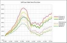
The S&P/Case–Shiller U.S. National Home Price Index is a composite of single-family home price indices for the nine U.S. Census divisions. It is calculated monthly, using a three-month moving average. The S&P national index is normalized to have a value of 100 in the January 2000.
The index kept by Shiller (available on his website at http://www.econ.yale.edu/~shiller/data.htm) is updated quarterly, and is normalized to have a value of 100 in 1890.
The composite and city indices

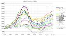
The S&P index family includes 20 metropolitan area indices and two composite indices as aggregates of the metropolitan areas. These indices are three-month moving averages. The composite and city indices are normalized to have a value of 100 in January 2000.
The indices are calculated monthly by Fiserv, Inc. — the company that owns and maintains the index and is published with a two-month lag on the last Tuesday of every month. Fiserv can provide a deeper view of home prices, at the ZIP code level beyond the 10 or 20 Metropolitan Statistical Area (MSA) view used by S&P.
Composite 10 index
CSXR is a composite index of the home price index for 10 major Metropolitan Statistical Areas in the United States. The index is published monthly by Standard & Poor's and uses the Case and Shiller method of a house price index using a modified version of the weighted-repeat sales methodology. This method is able to adjust for the quality of the homes sold, unlike simple indices based on averages. The CSXR is a three-month moving average as are the indices that compose it.
The following indexes are combined to create the CXSR composite index:
Composite 20 index
SPCS20R is a composite index of the home price index for 20 major Metropolitan Statistical Areas in the United States. The index is published monthly by Standard & Poor's and uses the Case and Shiller method of a house price index using a modified version of the weighted-repeat sales methodology. This method is able to adjust for the quality of the homes sold, unlike simple indices based on averages.
The following indexes are combined to create the SPCS20R composite index:
Correlations
Macromarkets.com reports the US index has a slightly negative correlation with stocks and bonds, but slightly positive correlation with commodities and Real Estate Investment Trusts (REIT).[11] REIT's track commercial real estate most closely, rather than home prices, explaining the low correlation.[12]
Historical values
Using Case and Shiller's original methods, the national index attained its all-time high of 198.01 in 2006 Q1. The S&P index attained its all-time high in July 2006, at a value of 206.52. On December 30, 2008, the index recorded its largest year-to-year drop. Since World War II, the original index has mostly fluctuated between 100 and 120, with peaks (followed by precipitous falls) in 1Q 1979 (which peaked at 122), 3Q 1989 (at 126), and 1Q 2006 (at 198). After the 2000s housing bubble, the low point of the index was in 1Q 2012, at 114. By 4Q 2013 the index had rebounded to 134.
 Case–Shiller home-price index from 1890 to 2012
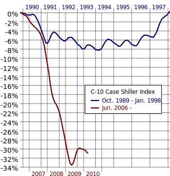
 Comparison the percentage change for the housing correction beginning in 2006 (red) and the correction (blue) beginning in 1989
| Selected Case–Shiller index values (from original data set back to 1890) | |||||
|---|---|---|---|---|---|
| YEAR | Annual/4Q | ||||
| 1890 | 100 | ||||
| 1900 | 101.57 | ||||
| 1910 | 93.11 | ||||
| 1920 | 66.07 | ||||
| 1930 | 69.49 | ||||
| 1940 | 81.73 | ||||
| 1950 | 105.89 | ||||
| 1960 | 109.65 | ||||
| 1970 | 109.56 | ||||
| 1975 | 103.46 | ||||
| 1979 | 118.82 | ||||
| 1984 | 105.44 | ||||
| 1989 | 124.89 | ||||
| 1994 | 108.33 | ||||
| 1996 | 106.73 | ||||
| 2000 | 123.30 | ||||
| 2005 | 195.35 | ||||
| 2006 | 192.29 | ||||
| 2007 | 170.09 | ||||
| 2008 | 133.97 | ||||
| 2009 | 130.93 | ||||
| 2010 | 124.56 | ||||
| 2011 | 115.84 | ||||
| 2012 | 121.58 | ||||
| 2013 | 134.02 | ||||
Securities tickers
Case–Shiller indexes are available for trading as futures and futures options.
Quotes are available from the CME.
| Ticker | Home Price Index description | MSA designation |
|---|---|---|
| CUS | Composite | A composite index of the top 10 MSAs in the country |
| LAX | Greater Los Angeles | Los Angeles–Long Beach–Santa Ana, CA |
| SDG | San Diego County, California | San Diego–Carlsbad–San Marcos, CA |
| SFR | San Francisco | San Francisco–Oakland–Fremont, CA |
| DEN | Denver-Aurora Metropolitan Area | Denver–Aurora, CO |
| WDC | Washington Metropolitan Area | Washington–Arlington–Alexandria, DC–VA–MD–WV |
| MIA | South Florida metropolitan area | Miami–Fort Lauderdale–Pompano Beach, FL |
| CHI | Chicago metropolitan area | Chicago–Naperville–Joliet, IL–IN–WI |
| BOS | Greater Boston | Boston–Cambridge–Quincy, MA |
| LAV | Las Vegas metropolitan area | Las Vegas–Paradise, NV MSA |
| NYM | New York metropolitan area | New York–Northern New Jersey–Long Island, NY–NJ–PA |
See also
References
- 1 2 3 Shiller, Robert (2005). Irrational Exuberance. Princeton University Press. p. 13. ISBN 0-691-12335-7.
- 1 2 3 4 5 Katie Benner (2009-07-07). "Bob Shiller didn't kill the housing market". CNNMoney.com. Retrieved 2009-07-07.
- ↑ Margaret Chadbourn (2013-04-25). "CoreLogic acquires Case–Shiller from Fiserv". Reuters.com. Retrieved 2013-05-07.
- ↑ http://www.cmegroup.com/trading/real-estate/files/spcaseshiller_fact_card.pdf
- ↑ Shiller, Robert (2005). Irrational Exuberance. Princeton University Press. p. 14. ISBN 0-691-12335-7.
- ↑ Shiller, Robert (2005). Irrational Exuberance. Princeton University Press. p. 19. ISBN 0-691-12335-7.
- 1 2 3 Shiller, Robert (2005). Irrational Exuberance. Princeton University Press. p. 22. ISBN 0-691-12335-7.
- ↑ Shiller, Robert. "Understanding recent trends in house prices and home ownership". National Bureau of Economic Research.
- 1 2 3 Shiller, Robert (2005). Irrational Exuberance. Princeton University Press. p. 16. ISBN 0-691-12335-7.
- ↑ Shiller, Robert (2005). Irrational Exuberance. Princeton University Press. p. 15. ISBN 0-691-12335-7.
- ↑ MacroMarkets at the Wayback Machine (archived March 28, 2007)
- ↑ Krantz, Matt (2011-05-26). "Can you invest in real estate using home price indexes?". USA Today.
- Mantell, Ruth (2008-12-30). "Home prices off record 18% in past year, Case–Shiller says". MarketWatch. Retrieved 2012-12-02.
External links
- CoreLogic Case–Shiller Indexes
- S&P/Case–Shiller Home Price Indices
- S&P's Blog on the Housing Market
- Shiller's online data website
- U.S. S&P/CS HPI Composite - 20 n.s.a. YoY