Bin (computational geometry)

The bin data structure.

A histogram ordered into 100,000 bins.

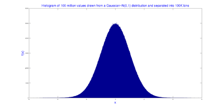
In computational geometry, the bin is a data structure which allows efficient region queries. Each time a data point falls into a bin, the frequency of that bin is increased by one.^[1]

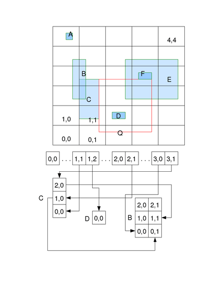
For example, if there are some axis-aligned rectangles on a 2D plane, answers the question: "Given a query rectangle, what are the rectangles intersecting it?". In the example in the figure, A, B, C, D, E and F are existing rectangles, the query with the rectangle Q should return C, D, E and F, if we define all rectangles as closed intervals.

The data structure partitions a region of the 2D plane into uniform-sized bins. The bounding box of the bins encloses all candidate rectangles to be queried. All the bins are arranged in a 2D array. All the candidates are represented also as 2D arrays. The size of a candidate's array is the number of bins it intersects. For example, in the figure, candidate B has 6 elements arranged in a 3 row by 2 column array because it intersects 6 bins in such an arrangement. Each bin contains the head of a singly linked list. If a candidate intersects a bin, it is chained to the bin's linked list. Each element in a candidate's array is a link node in the corresponding bin's linked list.

Operations

Query

From the query rectangle Q, we can find out which bin its lower-left corner intersects efficiently by simply subtracting the bin's bounding box's lower-left corner from the lower-left corner of Q and dividing the result by the width and height of a bin respectively. We then iterate the bins Q intersects and examine all the candidates in the linked-lists of these bins. For each candidate we check if it does indeed intersect Q. If so and it is not previously reported, then we report it. We can use the convention that we only report a candidate the first time we find it. This can be done easily by clipping the candidate against the query rectangle and comparing its lower-left corner against the current location. If it is a match then we report, otherwise we skip.

Insertion and deletion

Insertion is linear to the number of bins a candidate intersects because inserting a candidate into 1 bin is constant time. Deletion is more expensive because we need to search the singly linked list of each bin the candidate intersects.

In a multithread environment, insert, delete and query are mutually exclusive. However, instead of locking the whole data structure, a sub-range of bins may be locked. Detailed performance analysis should be done to justify the overhead.

Efficiency and tuning

The analysis is similar to a hash table. The worst-case scenario is that all candidates are concentrated in one bin. Then query is O(n), delete is O(n), and insert is O(1), where n is the number of candidates. If the candidates are evenly spaced so that each bin has a constant number of candidates, The query is O(k) where k is the number of bins the query rectangle intersects. Insert and delete are O(m) where m is the number of bins the inserting candidate intersects. In practice delete is much slower than insert.

Like a hash table, bin's efficiency depends a lot on the distribution of both location and size of candidates and queries. In general, the smaller the query rectangle, the more efficient the query. The bin's size should be such that it contains as few candidates as possible but large enough so that candidates do not span too many bins. If a candidate span many bins, a query has to skip this candidate over and over again after it is reported at the first bin of intersection. For example, in the figure, E is visited 4 times in the query of Q and so has to be skipped 3 times.

To further speed up the query, divisions can be replaced by right shifts. This requires the number of bins along an axis direction to be an exponent of 2.

Compared to other range query data structures

Against k-d tree, the bin structure allows efficient insertion and deletion without the complexity of rebalancing. This can be very useful in algorithms that need to incrementally add shapes to the search data structure.

References

↑ Harmony Search Optimization for HDR Prostate Brachytherapy. ProQuest. 2008.