Tensor derivative (continuum mechanics)
The derivatives of scalars, vectors, and second-order tensors with respect to second-order tensors are of considerable use in continuum mechanics. These derivatives are used in the theories of nonlinear elasticity and plasticity, particularly in the design of algorithms for numerical simulations.[1]
The directional derivative provides a systematic way of finding these derivatives.[2]
Derivatives with respect to vectors and second-order tensors
The definitions of directional derivatives for various situations are given below. It is assumed that the functions are sufficiently smooth that derivatives can be taken.
Derivatives of scalar valued functions of vectors
Let f(v) be a real valued function of the vector v. Then the derivative of f(v) with respect to v (or at v) in the direction u is the vector defined as
for all vectors u.
Properties:
1) If  then
then 
2) If  then
then 
3) If  then
then 
Derivatives of vector valued functions of vectors
Let f(v) be a vector valued function of the vector v. Then the derivative of f(v) with respect to v (or at v) in the direction u is the second order tensor defined as
for all vectors u.
- Properties:
- 1) If
 then
then 
- 2) If
 then
then 
- 3) If
 then
then 
Derivatives of scalar valued functions of second-order tensors
Let  be a real valued function of the second order tensor
  . Then the derivative of
  with respect to
  (or at
  ) in the direction
  is the second order tensor defined as
for all second order tensors  .
.
- Properties:
- 1) If
 then
then 
- 2) If
 then
then 
- 3) If
 then
then 
Derivatives of tensor valued functions of second-order tensors
Let  be a second order tensor valued function of the second order tensor
  . Then the derivative of
  with respect to
  (or at
  ) in the direction
  is the fourth order tensor defined as
for all second order tensors  .
.
- Properties:
- 1) If
 then
then 
- 2) If
 then
then 
- 3) If
 then
then 
- 4) If
 then
then 
Gradient of a tensor field
The gradient,  , of a tensor field
  in the direction of an arbitrary constant vector c is defined as:
The gradient of a tensor field of order n is a tensor field of order n+1.
Cartesian coordinates
- Note: the Einstein summation convention of summing on repeated indices is used below.
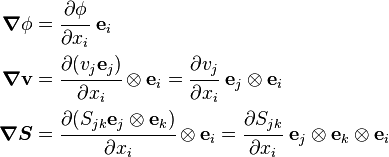
If  are the basis vectors in a Cartesian coordinate system, with coordinates of points denoted by (
 ), then the gradient of the tensor field
  is given by
Proof The vectors x and c can be written as
 and
and  . Let y := x + αc. In that case the gradient is given by
Since the basis vectors do not vary in a Cartesian coordinate system we have the following relations for the gradients of a scalar field  , a vector field v, and a second-order tensor field
  .
.
Curvilinear coordinates
- Note: the Einstein summation convention of summing on repeated indices is used below.
If  are the contravariant basis vectors in a curvilinear coordinate system, with coordinates of points denoted by (
 ), then the gradient of the tensor field
  is given by (see [3] for a proof.)
From this definition we have the following relations for the gradients of a scalar field  , a vector field v, and a second-order tensor field
  .
.
where the Christoffel symbol  is defined using
Cylindrical polar coordinates
In cylindrical coordinates, the gradient is given by
Divergence of a tensor field
The divergence of a tensor field  is defined using the recursive relation
where c is an arbitrary constant vector and v is a vector field. If  is a tensor field of order n > 1 then the divergence of the field is a tensor of order n−1.
Cartesian coordinates
- Note: the Einstein summation convention of summing on repeated indices is used below.
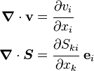
In a Cartesian coordinate system we have the following relations for a vector field v and a second-order tensor field  .
.
Note that last relation can be found in reference [4] under relation (1.14.13). Note also that according to the same paper in the case of the second-order tensor field, we have:
Curvilinear coordinates
- Note: the Einstein summation convention of summing on repeated indices is used below.
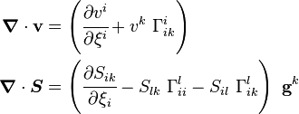
In curvilinear coordinates, the divergences of a vector field v and a second-order tensor field  are
are
Cylindrical polar coordinates
In cylindrical polar coordinates
Curl of a tensor field
The curl of an order-n > 1 tensor field  is also defined using the recursive relation
where c is an arbitrary constant vector and v is a vector field.
Curl of a first-order tensor (vector) field
Consider a vector field v and an arbitrary constant vector c. In index notation, the cross product is given by
where  is the permutation symbol. Then,
Therefore
Curl of a second-order tensor field
For a second-order tensor 
Hence, using the definition of the curl of a first-order tensor field,
Therefore, we have
Identities involving the curl of a tensor field
The most commonly used identity involving the curl of a tensor field,  , is
, is
This identity hold for tensor fields of all orders. For the important case of a second-order tensor,  , this identity implies that
Derivative of the determinant of a second-order tensor
The derivative of the determinant of a second order tensor  is given by
In an orthonormal basis, the components of  can be written as a matrix A. In that case, the right hand side corresponds the cofactors of the matrix.
Proof Let
 be a second order tensor and let
  . Then, from the definition of the derivative of a scalar valued function of a tensor, we have
Recall that we can expand the determinant of a tensor in the form of a characteristic equation in terms of the invariants
 using (note the sign of λ)
Using this expansion we can write
Recall that the invariant
 is given by
Hence,
Invoking the arbitrariness of
 we then have
Derivatives of the invariants of a second-order tensor
The principal invariants of a second order tensor are
The derivatives of these three invariants with respect to  are
are
Proof From the derivative of the determinant we know that For the derivatives of the other two invariants, let us go back to the characteristic equation
Using the same approach as for the determinant of a tensor, we can show that
Now the left hand side can be expanded as
Hence
or,
Expanding the right hand side and separating terms on the left hand side gives
or,
If we define
 and
and  , we can write the above as
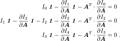
Collecting terms containing various powers of λ, we get
Then, invoking the arbitrariness of λ, we have
This implies that
Derivative of the second-order identity tensor
Let  be the second order identity tensor. Then the derivative of this tensor with respect to a second order tensor
  is given by
This is because  is independent of
  .
.
Derivative of a second-order tensor with respect to itself
Let  be a second order tensor. Then
Therefore,
Here  is the fourth order identity tensor. In index
notation with respect to an orthonormal basis
This result implies that
where
Therefore, if the tensor  is symmetric, then the derivative is also symmetric and
we get
where the symmetric fourth order identity tensor is
Derivative of the inverse of a second-order tensor
Let  and
and  be two second order tensors, then
In index notation with respect to an orthonormal basis
We also have
In index notation
If the tensor  is symmetric then
Proof Recall that Since
 , we can write
Using the product rule for second order tensors
we get
or,
Therefore,
Integration by parts
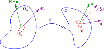
 , its boundary
  and the outward unit normal
Another important operation related to tensor derivatives in continuum mechanics is integration by parts. The formula for integration by parts can be written as
where  and
and  are differentiable tensor fields of arbitrary order,
  is the unit outward normal to the domain over which the tensor fields are defined,
  represents a generalized tensor product operator, and
  is a generalized gradient operator. When
  is equal to the identity tensor, we get the divergence theorem
We can express the formula for integration by parts in Cartesian index notation as
For the special case where the tensor product operation is a contraction of one index and the gradient operation is a divergence, and both  and
and  are second order tensors, we have
In index notation,
References
- ↑ J. C. Simo and T. J. R. Hughes, 1998, Computational Inelasticity, Springer
- ↑ J. E. Marsden and T. J. R. Hughes, 2000, Mathematical Foundations of Elasticity, Dover.
- ↑ Ogden, R. W., 2000, Nonlinear Elastic Deformations, Dover.
- ↑ http://homepages.engineering.auckland.ac.nz/~pkel015/SolidMechanicsBooks/Part_III/Chapter_1_Vectors_Tensors/Vectors_Tensors_14_Tensor_Calculus.pdf
![\frac{\partial f}{\partial \mathbf{v}}\cdot\mathbf{u} = Df(\mathbf{v})[\mathbf{u}] = \left[\frac{d }{d \alpha}~f(\mathbf{v} + \alpha~\mathbf{u})\right]_{\alpha = 0}](../I/m/eb463fc48503030f92e2a19717fcf271.png)
![\frac{\partial \mathbf{f}}{\partial \mathbf{v}}\cdot\mathbf{u} = D\mathbf{f}(\mathbf{v})[\mathbf{u}] = \left[\frac{d }{d \alpha}~\mathbf{f}(\mathbf{v} + \alpha~\mathbf{u} ) \right]_{\alpha = 0}](../I/m/e3b1106403d14044ef3ec71ef56c1d5e.png)
![\frac{\partial f}{\partial \boldsymbol{S}}:\boldsymbol{T} = Df(\boldsymbol{S})[\boldsymbol{T}] = \left[\frac{d }{d \alpha}~f(\boldsymbol{S} + \alpha~\boldsymbol{T})\right]_{\alpha = 0}](../I/m/301e4c30722d29c160fd62f552c72162.png)
![\frac{\partial \boldsymbol{F}}{\partial \boldsymbol{S}}:\boldsymbol{T} = D\boldsymbol{F}(\boldsymbol{S})[\boldsymbol{T}] = \left[\frac{d }{d \alpha}~\boldsymbol{F}(\boldsymbol{S} + \alpha~\boldsymbol{T})\right]_{\alpha = 0}](../I/m/f48a2042233fe78b410af72e4de27b5b.png)


![\begin{align}
\boldsymbol{\nabla}\boldsymbol{T}\cdot\mathbf{c} & = \left.\cfrac{d}{d\alpha}~\boldsymbol{T}(x_1+\alpha c_1, x_2 + \alpha c_2, x_3 + \alpha c_3)\right|_{\alpha=0} \equiv \left.\cfrac{d}{d\alpha}~\boldsymbol{T}(y_1, y_2, y_3)\right|_{\alpha=0} \\
& = \left [\cfrac{\partial{\boldsymbol{T}}}{\partial y_1}~\cfrac{\partial y_1}{\partial \alpha} + \cfrac{\partial{\boldsymbol{T}}}{\partial y_2}~\cfrac{\partial y_2}{\partial \alpha} +
\cfrac{\partial{\boldsymbol{T}}}{\partial y_3}~\cfrac{\partial y_3}{\partial \alpha} \right]_{\alpha=0} =
\left [\cfrac{\partial{\boldsymbol{T}}}{\partial y_1}~c_1 + \cfrac{\partial{\boldsymbol{T}}}{\partial y_2}~c_2 +
\cfrac{\partial{\boldsymbol{T}}}{\partial y_3}~c_3 \right]_{\alpha=0} \\
& = \cfrac{\partial{\boldsymbol{T}}}{\partial x_1}~c_1 + \cfrac{\partial{\boldsymbol{T}}}{\partial x_2}~c_2 +
\cfrac{\partial{\boldsymbol{T}}}{\partial x_3}~c_3 \equiv \cfrac{\partial{\boldsymbol{T}}}{\partial x_i}~c_i = \cfrac{\partial{\boldsymbol{T}}}{\partial x_i}~(\mathbf{e}_i\cdot\mathbf{c})
= \left[\mathbf{e}_i\otimes\cfrac{\partial{\boldsymbol{T}}}{\partial x_i}\right]\cdot\mathbf{c} \qquad \square
\end{align}](../I/m/1c7882514b21c5bad04e8841e1f1f2dd.png)


![\begin{align}
\boldsymbol{\nabla}\phi &=\cfrac{\partial \phi}{\partial r}~\mathbf{e}_r + \cfrac{1}{r}~\cfrac{\partial \phi}{\partial \theta}~\mathbf{e}_\theta +\cfrac{\partial \phi}{\partial z}~\mathbf{e}_z \\
\boldsymbol{\nabla}\mathbf{v} &= \cfrac{\partial v_r}{\partial r}~\mathbf{e}_r\otimes\mathbf{e}_r + \cfrac{1}{r}\left(\cfrac{\partial v_r}{\partial \theta} -v_\theta \right)~\mathbf{e}_r \otimes \mathbf{e}_\theta + \cfrac{\partial v_r}{\partial z}~\mathbf{e}_r\otimes\mathbf{e}_z +\cfrac{\partial v_\theta}{\partial r}~\mathbf{e}_\theta\otimes\mathbf{e}_r +\cfrac{1}{r}\left(\cfrac{\partial v_\theta}{\partial \theta} + v_r \right)~\mathbf{e}_\theta\otimes\mathbf{e}_\theta \\
&\quad + \cfrac{\partial v_\theta}{\partial z}~\mathbf{e}_\theta \otimes\mathbf{e}_z + \cfrac{\partial v_z}{\partial r}~\mathbf{e}_z\otimes\mathbf{e}_r + \cfrac{1}{r}\cfrac{\partial v_z}{\partial \theta}~\mathbf{e}_z \otimes\mathbf{e}_\theta + \cfrac{\partial v_z}{\partial z}~\mathbf{e}_z\otimes\mathbf{e}_z \\
\boldsymbol{\nabla}\boldsymbol{S} & = \frac{\partial S_{rr}}{\partial r}~\mathbf{e}_r\otimes\mathbf{e}_r\otimes\mathbf{e}_r + \cfrac{1}{r}\left[\frac{\partial S_{rr}}{\partial \theta} - (S_{\theta r}+S_{r\theta})\right]~\mathbf{e}_r\otimes\mathbf{e}_r\otimes\mathbf{e}_\theta + \frac{\partial S_{rr}}{\partial z}~\mathbf{e}_r \otimes \mathbf{e}_r\otimes\mathbf{e}_z + \frac{\partial S_{r\theta}}{\partial r}~\mathbf{e}_r\otimes\mathbf{e}_\theta\otimes\mathbf{e}_r \\
&\quad+ \cfrac{1}{r}\left[\frac{\partial S_{r\theta}}{\partial \theta} + (S_{rr}-S_{\theta\theta}) \right]~\mathbf{e}_r\otimes\mathbf{e}_\theta\otimes\mathbf{e}_\theta + \frac{\partial S_{r\theta}}{\partial z}~\mathbf{e}_r\otimes\mathbf{e}_\theta\otimes\mathbf{e}_z + \frac{\partial S_{rz}}{\partial r}~\mathbf{e}_r \otimes \mathbf{e}_z \otimes \mathbf{e}_r + \cfrac{1}{r}\left[\frac{\partial S_{rz}}{\partial \theta} -S_{\theta z} \right]~\mathbf{e}_r\otimes\mathbf{e}_z\otimes\mathbf{e}_\theta \\
&\quad+ \frac{\partial S_{rz}}{\partial z}~\mathbf{e}_r \otimes \mathbf{e}_z\otimes\mathbf{e}_z + \frac{\partial S_{\theta r}}{\partial r}~\mathbf{e}_\theta \otimes \mathbf{e}_r \otimes \mathbf{e}_r + \cfrac{1}{r}\left[\frac{\partial S_{\theta r}}{\partial \theta} + (S_{rr}-S_{\theta\theta}) \right]~\mathbf{e}_\theta\otimes\mathbf{e}_r\otimes\mathbf{e}_\theta + \frac{\partial S_{\theta r}}{\partial z}~\mathbf{e}_\theta\otimes\mathbf{e}_r\otimes\mathbf{e}_z \\
&\quad+ \frac{\partial S_{\theta\theta}}{\partial r}~\mathbf{e}_\theta\otimes\mathbf{e}_\theta\otimes\mathbf{e}_r +\cfrac{1}{r}\left[\frac{\partial S_{\theta\theta}}{\partial \theta} + (S_{r\theta}+S_{\theta r})\right]~\mathbf{e}_\theta\otimes\mathbf{e}_\theta\otimes\mathbf{e}_\theta + \frac{\partial S_{\theta\theta}}{\partial z}~\mathbf{e}_\theta \otimes \mathbf{e}_\theta \otimes \mathbf{e}_z + \frac{\partial S_{\theta z}}{\partial r}~\mathbf{e}_\theta \otimes \mathbf{e}_z\otimes\mathbf{e}_r \\
&\quad+ \cfrac{1}{r}\left[\frac{\partial S_{\theta z}}{\partial \theta} + S_{rz} \right]~\mathbf{e}_\theta \otimes\mathbf{e}_z\otimes\mathbf{e}_\theta + \frac{\partial S_{\theta z}}{\partial z}~\mathbf{e}_\theta\otimes\mathbf{e}_z\otimes\mathbf{e}_z + \frac{\partial S_{zr}}{\partial r}~\mathbf{e}_z\otimes\mathbf{e}_r\otimes\mathbf{e}_r + \cfrac{1}{r}\left[\frac{\partial S_{zr}}{\partial \theta} - S_{z\theta} \right]~\mathbf{e}_z \otimes \mathbf{e}_r \otimes\mathbf{e}_\theta \\
&\quad+ \frac{\partial S_{zr}}{\partial z}~\mathbf{e}_z\otimes\mathbf{e}_r\otimes\mathbf{e}_z + \frac{\partial S_{z\theta}}{\partial r}~\mathbf{e}_z \otimes \mathbf{e}_\theta \otimes \mathbf{e}_r + \cfrac{1}{r}\left[\frac{\partial S_{z\theta}}{\partial \theta} + S_{zr} \right]~\mathbf{e}_z \otimes\mathbf{e}_\theta \otimes \mathbf{e}_\theta + \frac{\partial S_{z\theta}}{\partial z}~\mathbf{e}_z\otimes\mathbf{e}_\theta\otimes\mathbf{e}_z \\
&\quad+ \frac{\partial S_{zz}}{\partial r}~\mathbf{e}_z\otimes\mathbf{e}_z\otimes\mathbf{e}_r + \cfrac{1}{r}~\frac{\partial S_{zz}}{\partial \theta }~\mathbf{e}_z \otimes \mathbf{e}_z \otimes\mathbf{e}_\theta + \frac{\partial S_{zz}}{\partial z}~\mathbf{e}_z\otimes\mathbf{e}_z\otimes\mathbf{e}_z
\end{align}](../I/m/40f29c56e66a57d8eccfa1b0989a06bd.png)


![\begin{align}
\boldsymbol{\nabla}\cdot\mathbf{v} &
= \cfrac{\partial v_r}{\partial r} +
\cfrac{1}{r}\left(\cfrac{\partial v_\theta}{\partial \theta} + v_r \right)
+ \cfrac{\partial v_z}{\partial z}\\
\boldsymbol{\nabla}\cdot\boldsymbol{S} &
= \frac{\partial S_{rr}}{\partial r}~\mathbf{e}_r
+ \frac{\partial S_{r\theta}}{\partial r}~\mathbf{e}_\theta
+ \frac{\partial S_{rz}}{\partial r}~\mathbf{e}_z \\
& +
\cfrac{1}{r}\left[\frac{\partial S_{\theta r}}{\partial \theta} + (S_{rr}-S_{\theta\theta})\right]~\mathbf{e}_r +
\cfrac{1}{r}\left[\frac{\partial S_{\theta\theta}}{\partial \theta} + (S_{r\theta}+S_{\theta r})\right]~\mathbf{e}_\theta +\cfrac{1}{r}\left[\frac{\partial S_{\theta z}}{\partial \theta} + S_{rz}\right]~\mathbf{e}_z \\
& +
\frac{\partial S_{zr}}{\partial z}~\mathbf{e}_r +
\frac{\partial S_{z\theta}}{\partial z}~\mathbf{e}_\theta +
\frac{\partial S_{zz}}{\partial z}~\mathbf{e}_z
\end{align}](../I/m/83beb9260e523fae665f7817e0b16d42.png)


![\frac{\partial }{\partial \boldsymbol{A}}\det(\boldsymbol{A}) = \det(\boldsymbol{A})~[\boldsymbol{A}^{-1}]^T ~.](../I/m/388dc10a74be0c3a8cb93c6e1ea20661.png)
![\begin{align}
\frac{\partial f}{\partial \boldsymbol{A}}:\boldsymbol{T} & = \left.\cfrac{d}{d\alpha} \det(\boldsymbol{A} + \alpha~\boldsymbol{T}) \right|_{\alpha=0} \\
& = \left.\cfrac{d}{d\alpha} \det\left[\alpha~\boldsymbol{A}\left(\cfrac{1}{\alpha}~\boldsymbol{\mathit{I}} + \boldsymbol{A}^{-1}\cdot\boldsymbol{T}\right) \right] \right|_{\alpha=0} \\
& = \left.\cfrac{d}{d\alpha} \left[\alpha^3~\det(\boldsymbol{A})~\det\left(\cfrac{1}{\alpha}~\boldsymbol{\mathit{I}} + \boldsymbol{A}^{-1} \cdot \boldsymbol{T}\right)\right]\right|_{\alpha=0}.
\end{align}](../I/m/d49f590a9b20bdb78de6312637e25440.png)

![\begin{align}
\frac{\partial f}{\partial \boldsymbol{A}}:\boldsymbol{T}
& = \left.\cfrac{d}{d\alpha} \left[\alpha^3~\det(\boldsymbol{A})~
\left(\cfrac{1}{\alpha^3} + I_1(\boldsymbol{A}^{-1}\cdot\boldsymbol{T})~\cfrac{1}{\alpha^2} +
I_2(\boldsymbol{A}^{-1}\cdot\boldsymbol{T})~\cfrac{1}{\alpha} + I_3(\boldsymbol{A}^{-1}\cdot\boldsymbol{T})\right)
\right] \right|_{\alpha=0} \\
& = \left.\det(\boldsymbol{A})~\cfrac{d}{d\alpha} \left[
1 + I_1(\boldsymbol{A}^{-1}\cdot\boldsymbol{T})~\alpha +
I_2(\boldsymbol{A}^{-1}\cdot\boldsymbol{T})~\alpha^2 + I_3(\boldsymbol{A}^{-1}\cdot\boldsymbol{T})~\alpha^3
\right] \right|_{\alpha=0} \\
& = \left.\det(\boldsymbol{A})~\left[I_1(\boldsymbol{A}^{-1}\cdot\boldsymbol{T}) +
2~I_2(\boldsymbol{A}^{-1}\cdot\boldsymbol{T})~\alpha + 3~I_3(\boldsymbol{A}^{-1}\cdot\boldsymbol{T})~\alpha^2
\right] \right|_{\alpha=0} \\
& = \det(\boldsymbol{A})~I_1(\boldsymbol{A}^{-1}\cdot\boldsymbol{T}) ~.
\end{align}](../I/m/7f31e3d92a4861d3e8592cf9b79f25c4.png)

![\frac{\partial f}{\partial \boldsymbol{A}}:\boldsymbol{T} = \det(\boldsymbol{A})~\text{tr}(\boldsymbol{A}^{-1}\cdot\boldsymbol{T})= \det(\boldsymbol{A})~[\boldsymbol{A}^{-1}]^T : \boldsymbol{T}.](../I/m/61a8ca769f9fbfda2aabfdbf07bc0a3b.png)
![\frac{\partial f}{\partial \boldsymbol{A}} = \det(\boldsymbol{A})~[\boldsymbol{A}^{-1}]^T ~.](../I/m/2f7e0ee3edd0598e34322e34630272b6.png)
![\begin{align}
I_1(\boldsymbol{A}) & = \text{tr}{\boldsymbol{A}} \\
I_2(\boldsymbol{A}) & = \frac{1}{2} \left[ (\text{tr}{\boldsymbol{A}})^2 - \text{tr}{\boldsymbol{A}^2} \right] \\
I_3(\boldsymbol{A}) & = \det(\boldsymbol{A})
\end{align}](../I/m/f77d412e4977c723a2f483f734d1f673.png)
![\begin{align}
\frac{\partial I_1}{\partial \boldsymbol{A}} & = \boldsymbol{\mathit{1}} \\
\frac{\partial I_2}{\partial \boldsymbol{A}} & = I_1~\boldsymbol{\mathit{1}} - \boldsymbol{A}^T \\
\frac{\partial I_3}{\partial \boldsymbol{A}} & = \det(\boldsymbol{A})~[\boldsymbol{A}^{-1}]^T
= I_2~\boldsymbol{\mathit{1}} - \boldsymbol{A}^T~(I_1~\boldsymbol{\mathit{1}} - \boldsymbol{A}^T)
= (\boldsymbol{A}^2 - I_1~\boldsymbol{A} + I_2~\boldsymbol{\mathit{1}})^T
\end{align}](../I/m/00e1300ec05d7463f46e75b35bb3a8f0.png)
![\frac{\partial I_3}{\partial \boldsymbol{A}} = \det(\boldsymbol{A})~[\boldsymbol{A}^{-1}]^T ~.](../I/m/9ae06d0eb9e59c6da04e332bc5bfe178.png)

![\frac{\partial }{\partial \boldsymbol{A}}\det(\lambda~\boldsymbol{\mathit{1}} + \boldsymbol{A}) =
\det(\lambda~\boldsymbol{\mathit{1}} + \boldsymbol{A})~[(\lambda~\boldsymbol{\mathit{1}}+\boldsymbol{A})^{-1}]^T ~.](../I/m/d01e8a7c8603447f3843a6b580ca2e34.png)
![\begin{align}
\frac{\partial }{\partial \boldsymbol{A}}\det(\lambda~\boldsymbol{\mathit{1}} + \boldsymbol{A}) & =
\frac{\partial }{\partial \boldsymbol{A}}\left[
\lambda^3 + I_1(\boldsymbol{A})~\lambda^2 + I_2(\boldsymbol{A})~\lambda + I_3(\boldsymbol{A}) \right] \\
& =
\frac{\partial I_1}{\partial \boldsymbol{A}}~\lambda^2 + \frac{\partial I_2}{\partial \boldsymbol{A}}~\lambda +
\frac{\partial I_3}{\partial \boldsymbol{A}}~.
\end{align}](../I/m/7dacdc0c1310bcc7f3935a978c120ebc.png)
![\frac{\partial I_1}{\partial \boldsymbol{A}}~\lambda^2 + \frac{\partial I_2}{\partial \boldsymbol{A}}~\lambda +
\frac{\partial I_3}{\partial \boldsymbol{A}} =
\det(\lambda~\boldsymbol{\mathit{1}} + \boldsymbol{A})~[(\lambda~\boldsymbol{\mathit{1}}+\boldsymbol{A})^{-1}]^T](../I/m/2d6fc66a3bd521bf023aed6414e0d387.png)
![(\lambda~\boldsymbol{\mathit{1}}+\boldsymbol{A})^T\cdot\left[
\frac{\partial I_1}{\partial \boldsymbol{A}}~\lambda^2 + \frac{\partial I_2}{\partial \boldsymbol{A}}~\lambda +
\frac{\partial I_3}{\partial \boldsymbol{A}}\right] =
\det(\lambda~\boldsymbol{\mathit{1}} + \boldsymbol{A})~\boldsymbol{\mathit{1}} ~.](../I/m/d3c98ee96a3a8a952eec91120a23e289.png)
![(\lambda~\boldsymbol{\mathit{1}} +\boldsymbol{A}^T)\cdot\left[
\frac{\partial I_1}{\partial \boldsymbol{A}}~\lambda^2 + \frac{\partial I_2}{\partial \boldsymbol{A}}~\lambda +
\frac{\partial I_3}{\partial \boldsymbol{A}}\right] =
\left[\lambda^3 + I_1~\lambda^2 + I_2~\lambda + I_3\right]
\boldsymbol{\mathit{1}}](../I/m/c0fcb3a6f568caab09717b59ad5d3588.png)
![\begin{align}
\left[\frac{\partial I_1}{\partial \boldsymbol{A}}~\lambda^3 \right.&
\left.+ \frac{\partial I_2}{\partial \boldsymbol{A}}~\lambda^2 +
\frac{\partial I_3}{\partial \boldsymbol{A}}~\lambda\right]\boldsymbol{\mathit{1}} +
\boldsymbol{A}^T\cdot\frac{\partial I_1}{\partial \boldsymbol{A}}~\lambda^2 +
\boldsymbol{A}^T\cdot\frac{\partial I_2}{\partial \boldsymbol{A}}~\lambda +
\boldsymbol{A}^T\cdot\frac{\partial I_3}{\partial \boldsymbol{A}} \\
& =
\left[\lambda^3 + I_1~\lambda^2 + I_2~\lambda + I_3\right]
\boldsymbol{\mathit{1}} ~.
\end{align}](../I/m/3e67aa96282a5dd15b16bf99cc073f4f.png)
![\begin{align}
\left[\frac{\partial I_1}{\partial \boldsymbol{A}}~\lambda^3 \right.&
\left.+ \frac{\partial I_2}{\partial \boldsymbol{A}}~\lambda^2 +
\frac{\partial I_3}{\partial \boldsymbol{A}}~\lambda + \frac{\partial I_4}{\partial \boldsymbol{A}}\right]\boldsymbol{\mathit{1}} +
\boldsymbol{A}^T\cdot\frac{\partial I_0}{\partial \boldsymbol{A}}~\lambda^3 +
\boldsymbol{A}^T\cdot\frac{\partial I_1}{\partial \boldsymbol{A}}~\lambda^2 +
\boldsymbol{A}^T\cdot\frac{\partial I_2}{\partial \boldsymbol{A}}~\lambda +
\boldsymbol{A}^T\cdot\frac{\partial I_3}{\partial \boldsymbol{A}} \\
&=
\left[I_0~\lambda^3 + I_1~\lambda^2 + I_2~\lambda + I_3\right]
\boldsymbol{\mathit{1}} ~.
\end{align}](../I/m/8ce6b3400ae926be35b5957de3be6d01.png)



![\frac{\partial \boldsymbol{A}}{\partial \boldsymbol{A}}:\boldsymbol{T} = \left[\frac{\partial }{\partial \alpha} (\boldsymbol{A} + \alpha~\boldsymbol{T})\right]_{\alpha = 0} = \boldsymbol{T} = \boldsymbol{\mathsf{I}}:\boldsymbol{T}](../I/m/952a2c48344aada7948136a9246f697c.png)


![\frac{\partial }{\partial \boldsymbol{S}}[\boldsymbol{F}_1(\boldsymbol{S})\cdot\boldsymbol{F}_2(\boldsymbol{S})]:\boldsymbol{T} =
\left(\frac{\partial \boldsymbol{F}_1}{\partial \boldsymbol{S}}:\boldsymbol{T}\right)\cdot\boldsymbol{F}_2 +
\boldsymbol{F}_1\cdot\left(\frac{\partial \boldsymbol{F}_2}{\partial \boldsymbol{S}}:\boldsymbol{T}\right)](../I/m/96bb99e98d6719745485b79b63d25198.png)


