Shearlet

In applied mathematical analysis, shearlets are a multiscale framework which allows to efficiently encode anisotropic features in multivariate problem classes. Originally, shearlets were introduced in 2006 ^[1] for the analysis as well as sparse approximation of functions $f \in L^2(\R^2)$ . They are a natural extension of wavelets to accommodate the fact that multivariate functions are typically governed by anisotropic features such as edges in images, however, wavelets as isotropic objects are not capable of capturing such phenomena.

Shearlets are constructed by parabolic scaling, shearing and translation applied to a few generating functions. At fine scales, they are essentially supported within skinny and directional ridges following the parabolic scaling law, which reads length² ≈ width. Similar to wavelets, shearlets arise from the affine group and allow a unified treatment of the continuum and digital situation leading to faithful implementations. Although they do not constitute an orthonormal basis for $L^2(\R^2)$ , they still form a frame allowing stable expansions of arbitrary functions $f \in L^2(\R^2)$ .

One of the most important properties of shearlets is the fact that they provide optimally sparse approximations (in the sense of optimality in ^[2]) for cartoon-like functions $f$ . In imaging sciences, cartoon-like functions serve as a model for anisotropic features and are compactly supported in $[0,1]^2$ while being $C^2$ apart from a closed piecewise $C^2$ singularity curve with bounded curvature. The decay rate of the $L^2$ -error of the $N$ -term shearlet approximation obtained by taking the $N$ largest coefficients from the shearlet expansion is in fact optimal up to a log-factor:^[3]^[4]

\| f - f_N \|_{L^2}^2 \leq C N^{-2} (\log N)^3, \quad N \to \infty,

where the constant $C$ depends only on the maximum curvature of the singularity curve and the maximum magnitudes of $f$ , $f^{'}$ and $f^{''}$ . This approximation rate significantly improves the best $N$ -term approximation rate of wavelets providing only $O(N^{-1})$ for such class of functions.

Shearlets are to date the only directional representation system which provides sparse approximation of anisotropic features while providing a unified treatment of the continuum and digital realm in the sense of allowing faithful implementation. Extensions of shearlet systems to $L^2(\R^d), d \ge 2$ are also available. A comprehensive presentation of the theory and applications of shearlets can be found in: ^[5]

Definition

Continuous shearlet systems

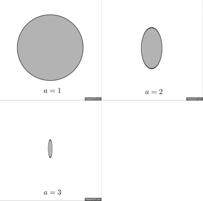
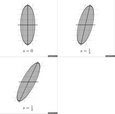
Geometric effects of parabolic scaling and shearing with several parameters a and s.

The construction of continuous shearlet systems is based on parabolic scaling matrices

A_a = \begin{bmatrix} a & 0 \\ 0 & a^{1/2} \end{bmatrix}, \quad a > 0

as a mean to change the resolution, on shear matrices

S_s = \begin{bmatrix} 1 & s \\ 0 & 1 \end{bmatrix}, \quad s \in \R

as a means to change the orientation, and finally on translations to change the positioning. In comparison to curvelets, shearlets use shearings instead of rotations, the advantage being that the shear operator $S_s$ leaves the integer lattice invariant in case $s \in \Z$ , i.e., $S_s \Z^2 \subseteq \Z^2.$ This indeed allows a unified treatment of the continuum and digital realm, thereby guaranteeing a faithful digital implementation.

For $\psi \in L^2(\R^2)$ the continuous shearlet system generated by $\psi$ is then defined as

\operatorname{SH}_{\mathrm{cont}}(\psi) = \{ \psi_{a,s,t} = a^{3/4} \psi(S_s A_a (\cdot - t)) \mid a > 0, s \in \R, t \in \R^2 \},

and the corresponding continuous shearlet transform is given by the map

f \mapsto \mathcal{SH}_\psi f(a, s, t) = \langle f, \psi_{a,s,t} \rangle, \quad f \in L^2(\R^2), \quad (a, s, t) \in \R_{>0} \times \R \times \R^2.

Discrete shearlet systems

A discrete version of shearlet systems can be directly obtained from $\operatorname{SH}_{\mathrm{cont}}(\psi)$ by discretizing the parameter set $\R_{>0} \times \R \times \R^2.$ There are numerous approaches for this but the most popular one is given by

\{ (2^j, k, A_{2^j}^{-1} S_k^{-1} m) \mid j \in \Z, k \in \Z, m \in \Z^2\} \subseteq \R_{>0} \times \R \times \R^2.

From this, the discrete shearlet system associated with the shearlet generator $\psi$ is defined by

\operatorname{SH}(\psi) = \{ \psi_{j,k,m} = 2^{3j/4} \psi(S_k A_{2^j} \cdot{} - m) \mid j \in \Z, k \in \Z, m \in \Z^2 \},

and the associated discrete shearlet transform is defined by

f \mapsto \mathcal{SH}_\psi f(j, k, m) = \langle f, \psi_{j,k,m} \rangle, \quad f \in L^2(\R^2), \quad (j, k, m) \in \Z \times \Z \times \Z^2.

Examples

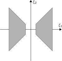
Trapezoidal frequency support of the classical shearlet.

Frequency tiling of the (discrete) classical shearlet system.

Let $\psi_1 \in L^2(\R)$ be a function satisfying the discrete Calderón condition, i.e.,

\sum_{j \in \Z} |\hat\psi_1(2^{-j} \xi)|^2 = 1, \quad \xi \in \R,

with $\hat\psi_1 \in C^\infty(\R)$ and $\operatorname{supp}\hat\psi_1 \subseteq [-\tfrac{1}{2}, -\tfrac{1}{16}] \cup [\tfrac{1}{16}, \tfrac{1}{2}],$ where $\hat\psi_1$ denotes the Fourier transform of $\psi_1.$ For instance, one can choose $\psi_1$ to be a Meyer wavelet. Furthermore, let $\psi_2 \in L^2(\R)$ be such that $\hat\psi_2 \in C^\infty(\R),$ $\operatorname{supp}\hat\psi_2 \subseteq [-1, 1]$ and

\sum_{k \in Z} |\hat\psi_2(\xi + k)|^2 = 1, \quad \xi \in \R.

One typically chooses $\hat \psi_2$ to be a smooth bump function. Then $\psi \in L^2(\R^2)$ given by

\hat\psi(\xi) = \hat\psi_1(\xi_1) \hat\psi_2\left( \tfrac{\xi_2}{\xi_1} \right), \quad \xi = (\xi_1, \xi_2) \in \R^2,

is called a classical shearlet. It can be shown that the corresponding discrete shearlet system $\operatorname{SH}(\psi)$ constitutes a Parseval frame for $L^2(\R^2)$ consisting of bandlimited functions.^[5]

Another example are compactly supported shearlet systems, where a compactly supported function $\psi \in L^2(\R^2)$ can be chosen so that $\operatorname{SH}(\psi)$ forms a frame for $L^2(\R^2)$ .^[4]^[6]^[7]^[8] In this case, all shearlet elements in $\operatorname{SH}(\psi)$ are compactly supported providing superior spatial localization compared to the classical shearlets, which are bandlimited. Although a compactly supported shearlet system does not generally form a Parseval frame, any function $f \in L^2(\R^2)$ can be represented by the shearlet expansion due to its frame property.

Cone-adapted shearlets

One drawback of shearlets defined as above is the directional bias of shearlet elements associated with large shearing parameters. This effect is already recognizable in the frequency tiling of classical shearlets (see Figure in Section #Examples), where the frequency support of a shearlet increasingly aligns along the $\xi_2$ -axis as the shearing parameter $s$ goes to infinity. This causes serious problems when analyzing a function whose Fourier transform is concentrated around the $\xi_2$ -axis.

Decomposition of the frequency domain into cones.

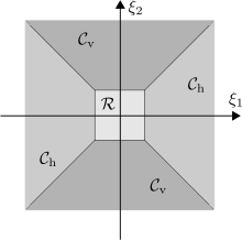
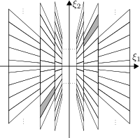
To deal with this problem, the frequency domain is divided into a low-frequency part and two conic regions (see Figure):

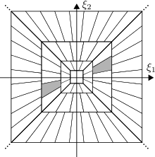
\begin{align} \mathcal{R} &= \left\{ (\xi_1, \xi_2) \in \R^2 \mid |\xi_1|, |\xi_2| \leq 1 \right\}, \\ \mathcal{C}_{\mathrm{h}} &= \left\{ (\xi_1, \xi_2) \in \R^2 \mid | \xi_2 / \xi_1 | \leq 1, |\xi_1| > 1 \right\}, \\ \mathcal{C}_{\mathrm{v}} &= \left\{ (\xi_1, \xi_2) \in \R^2 \mid | \xi_1 / \xi_2 | \leq 1, |\xi_2| > 1 \right\}. \end{align}

Frequency tiling of the cone-adapted shearlet system generated by the classical shearlet.

The associated cone-adapted discrete shearlet system consists of three parts, each one corresponding to one of these frequency domains. It is generated by three functions $\phi, \psi, \tilde\psi \in L^2(\R^2)$ and a lattice sampling factor $c = (c_1, c_2) \in (\R_{> 0})^2:$

\operatorname{SH}(\phi, \psi, \tilde\psi; c) = \Phi(\phi; c_1) \cup \Psi(\psi; c) \cup \tilde\Psi(\tilde\psi; c),

where

\begin{align} \Phi(\phi; c_1) &= \{ \phi_m = \phi(\cdot{} - c_1 m) \mid m \in \Z^2 \}, \\ \Psi(\psi; c) &= \{ \psi_{j,k,m} = 2^{3j/4} \psi(S_k A_{2^j} \cdot{} - M_c m) \mid j \geq 0, |k| \leq \lceil 2^{j/2} \rceil, m \in \Z^2 \}, \\ \tilde\Psi(\tilde\psi; c) &= \{ \tilde{\psi}_{j,k,m} = 2^{3j/4} \psi(\tilde{S}_k \tilde{A}_{2^j} \cdot{} - \tilde{M}_c m) \mid j \geq 0, |k| \leq \lceil 2^{j/2} \rceil, m \in \Z^2 \}, \end{align}

with

\begin{align} & \tilde{A}_a = \begin{bmatrix} a^{1/2} & 0 \\ 0 & a \end{bmatrix}, \; a > 0, \quad \tilde{S}_s = \begin{bmatrix} 1 & 0 \\ s & 1 \end{bmatrix}, \; s \in \R, \quad M_c = \begin{bmatrix} c_1 & 0 \\ 0 & c_2 \end{bmatrix}, \quad \text{and} \quad \tilde{M}_c = \begin{bmatrix} c_2 & 0 \\ 0 & c_1 \end{bmatrix}. \end{align}

The systems $\Psi(\psi)$ and $\tilde\Psi(\tilde\psi)$ basically differ in the reversed roles of $x_1$ and $x_2$ . Thus, they correspond to the conic regions $\mathcal{C}_{\mathrm{h}}$ and $\mathcal{C}_{\mathrm{v}}$ , respectively. Finally, the scaling function $\phi$ is associated with the low-frequency part $\mathcal{R}$ .

Applications

Image processing and computer sciences ^[5]
- Denoising
- Inverse problems
- Image enhancement
- Edge detection
- Inpainting
- Image separation
PDEs ^[5]
- Resolution of the wavefront set
- Transport equations
Coorbit theory, characterization of smoothness spaces ^[5]
Differential geometry: manifold learning

Generalizations and extensions

3D-Shearlets ^[7]^[9]
$\alpha$ -Shearlets ^[7]
Parabolic molecules ^[10]

References

↑ Guo, Kanghui, Gitta Kutyniok, and Demetrio Labate. "Sparse multidimensional representations using anisotropic dilation and shear operators." Wavelets and Splines (Athens, GA, 2005), G. Chen and MJ Lai, eds., Nashboro Press, Nashville, TN (2006): 189–201. PDF PDF
↑ Donoho, David Leigh. "Sparse components of images and optimal atomic decompositions." Constructive Approximation 17.3 (2001): 353–382. PDF PDF
↑ Guo, Kanghui, and Demetrio Labate. "Optimally sparse multidimensional representation using shearlets." SIAM Journal on Mathematical Analysis 39.1 (2007): 298–318. PDF PDF
1 2 Kutyniok, Gitta, and Wang-Q Lim. "Compactly supported shearlets are optimally sparse." Journal of Approximation Theory 163.11 (2011): 1564–1589. PDF PDF
1 2 3 4 5 Kutyniok, Gitta, and Demetrio Labate, eds. Shearlets: Multiscale analysis for multivariate data. Springer, 2012, ISBN 0-8176-8315-1
↑ Kittipoom, Pisamai, Gitta Kutyniok, and Wang-Q Lim. "Construction of compactly supported shearlet frames." Constructive Approximation 35.1 (2012): 21–72. PDF PDF
1 2 3 Kutyniok, Gitta, Jakob Lemvig, and Wang-Q Lim. "Optimally sparse approximations of 3D functions by compactly supported shearlet frames." SIAM Journal on Mathematical Analysis 44.4 (2012): 2962–3017. PDF PDF
↑ Purnendu Banerjee and B. B. Chaudhuri, “Video Text Localization using Wavelet and Shearlet Transforms”, In Proc. SPIE 9021, Document Recognition and Retrieval XXI, 2014 (doi:10.1117/12.2036077).PDF PDF
↑ Guo, Kanghui, and Demetrio Labate. "The construction of smooth Parseval frames of shearlets." Mathematical Modelling of Natural Phenomena 8.01 (2013): 82–105. PDF PDF
↑ Grohs, Philipp and Kutyniok, Gitta. "Parabolic molecules." Foundations of Computational Mathematics (to appear) PDF PDF

External links

This article is issued from Wikipedia - version of the Monday, December 21, 2015. The text is available under the Creative Commons Attribution/Share Alike but additional terms may apply for the media files.