Semidefinite embedding
Semidefinite embedding (SDE) or maximum variance unfolding (MVU) is an algorithm in computer science that uses semidefinite programming to perform non-linear dimensionality reduction of high-dimensional vectorial input data. MVU can be viewed as a non-linear generalization of Principal component analysis.
Non-linear dimensionality reduction algorithms attempt to map high-dimensional data onto a low-dimensional Euclidean vector space. Maximum variance Unfolding is a member of the manifold learning family, which also include algorithms such as isomap and locally linear embedding. In manifold learning, the input data is assumed to be sampled from a low dimensional manifold that is embedded inside of a higher-dimensional vector space. The main intuition behind MVU is to exploit the local linearity of manifolds and create a mapping that preserves local neighborhoods at every point of the underlying manifold.
MVU creates a mapping from the high dimensional input vectors to some low dimensional Euclidean vector space in the following steps:
A neighborhood graph is created. Each input is connected with its k-nearest input vectors (according to Euclidean distance metric) and all k-nearest neighbors are connected with each other. If the data is sampled well enough, the resulting graph is a discrete approximation of the underlying manifold.
The neighborhood graph is "unfolded" with the help of semidefinite programming. Instead of learning the output vectors directly, the semidefinite programming aims to find an inner product matrix that maximizes the pairwise distances between any two inputs that are not connected in the neighborhood graph while preserving the nearest neighbors distances.
The low-dimensional embedding is finally obtained by application of multidimensional scaling on the learned inner product matrix.
The steps of applying semidefinite programming followed by a linear dimensionality reduction step to recover a low-dimensional embedding into a Euclidean space were first proposed by Linial, London, and Rabinovich.
Optimization Formulation
Let  be the original input and
  be the embedding. If
  are two neighbors, then the local isometry constraint that needs to be satisfied is:
Let  be the Gram matrices of
  and
and  (i.e.:
  ). We can express the above constraint for every neighbor points
  in term of
  :
:
In addition, we also want to constrain the embedding  to center at the origin:

As described above, except the distances of neighbor points are preserved, the algorithm aims to maximize the pairwise distance of every pair of points. The objective function to be maximized is:

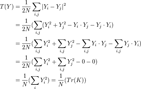
Intuitively, maximizing the function above is equivalent to pulling the points as far away from each other as possible and therefore "unfold" the manifold. The local isometry constraint prevents the objective function from going to infinity. Proof:
Let  where
where  if i and j are neighbors and
  otherwise.
Since the graph has N points, the distance between any two points  . We can then bound the objective function as follow:
The objective function can be rewritten purely in the form of the Gram matrix:
Finally, the optimization can be formulated as:
Maximize 
Subject to  and
and
 where
where 
After the Gram matrix  is learned by semidefinite programming, the output
  can be obtained via Cholesky decomposition. In particular, the Gram matrix can be written as
  where
where  is the i-th element of eigenvector
  of the eigenvalue
  .
.
It follows that the  -th element of the output
  is
is  .
.
Comparison to other methods
Semidefinite embedding is much better in revealing the underlying dimension of the data compared to LLE and Laplacian eigenmaps. It also guarantees that the nearest neighbors in the embedding is the same as the original nearest neighbor for each point while the other two methods do not. On the other hand, semidefinite embedding is much slower and harder to scale to large data.
Semidefinite embedding outperforms Isomap when the manifold is not a convex subset of the Euclidean space.
See also
References
- Unsupervised learning of image manifolds by semidefinite programming K. Q. Weinberger and L. K. Saul (2004). In Proceedings of the IEEE Conference on Computer Vision and Pattern Recognition (CVPR-04), Washington D.C.
- Unsupervised learning of image manifolds by semidefinite programming K. Q. Weinberger and L. K. Saul (2005), International Journal of Computer Vision - In Special Issue: Computer Vision and Pattern Recognition-CVPR 2005 Guest Editor(s): Aaron Bobick, Rama Chellappa, Larry Davis, pages 77–90, Volume 70, Number 1, Springer Netherlands
- The geometry of graphs and some of its algorithmic applications, Nathan Linial, Eran London, Yuri Rabinovich, IEEE Symposium on Foundations of Computer Science.


