Runge–Kutta methods

In numerical analysis, the Runge–Kutta methods are a family of implicit and explicit iterative methods used in temporal discretization for the approximate solutions of ordinary differential equations. These methods were developed around 1900 by the German mathematicians C. Runge and M. W. Kutta.

See the article on numerical methods for ordinary differential equations for more background and other methods. See also List of Runge–Kutta methods.

The Runge–Kutta method

One member of the family of Runge–Kutta methods is often referred to as "RK4", "classical Runge–Kutta method" or simply as "the Runge–Kutta method".

Let an initial value problem be specified as follows.

\dot{y} = f(t, y), \quad y(t_0) = y_0.

Here, y is an unknown function (scalar or vector) of time t which we would like to approximate; we are told that $\dot{y}$ , the rate at which y changes, is a function of t and of y itself. At the initial time $t_0$ the corresponding y-value is $y_0$ . The function f and the data $t_0$ , $y_0$ are given.

Now pick a step-size h>0 and define

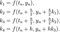
\begin{align} y_{n+1} &= y_n + \tfrac{h}{6}\left(k_1 + 2k_2 + 2k_3 + k_4 \right)\\ t_{n+1} &= t_n + h \\ \end{align}

for n = 0, 1, 2, 3, . . . , using

\begin{align} k_1 &= f(t_n, y_n), \\ k_2 &= f(t_n + \tfrac{h}{2}, y_n + \tfrac{h}{2} k_1), \\ k_3 &= f(t_n + \tfrac{h}{2}, y_n + \tfrac{h}{2} k_2), \\ k_4 &= f(t_n + h, y_n + hk_3). \end{align}

^[1]

(Note: the above equations have different but equivalent definitions in different texts).^[2]

Here $y_{n+1}$ is the RK4 approximation of $y(t_{n+1})$ , and the next value ( $y_{n+1}$ ) is determined by the present value ( $y_n$ ) plus the weighted average of four increments, where each increment is the product of the size of the interval, h, and an estimated slope specified by function f on the right-hand side of the differential equation.

$k_1$ is the increment based on the slope at the beginning of the interval, using ${y}$ , (Euler's method) ;
$k_2$ is the increment based on the slope at the midpoint of the interval, using ${y} + \tfrac{h}{2}k_1$ ;
$k_3$ is again the increment based on the slope at the midpoint, but now using ${y} + \tfrac{h}{2}k_2$ ;
$k_4$ is the increment based on the slope at the end of the interval, using ${y} + hk_3$ .

In averaging the four increments, greater weight is given to the increments at the midpoint. If $f$ is independent of $y$ , so that the differential equation is equivalent to a simple integral, then RK4 is Simpson's rule.^[3]

The RK4 method is a fourth-order method, meaning that the local truncation error is on the order of $O(h^5)$ , while the total accumulated error is order $O(h^4)$ .

Explicit Runge–Kutta methods

The family of explicit Runge–Kutta methods is a generalization of the RK4 method mentioned above. It is given by

y_{n+1} = y_n + h \sum_{i=1}^s b_i k_i,

where

k_1 = f(t_n, y_n), \,

k_2 = f(t_n+c_2h, y_n+h(a_{21}k_1)), \,

k_3 = f(t_n+c_3h, y_n+h(a_{31}k_1+a_{32}k_2)), \,

\vdots

k_s = f(t_n+c_sh, y_n+h(a_{s1}k_1+a_{s2}k_2+\cdots+a_{s,s-1}k_{s-1})).

^[4]

(Note: the above equations have different but equivalent definitions in different texts).^[2]

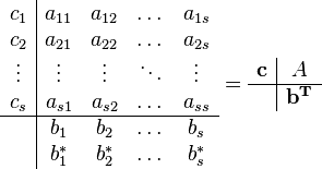
To specify a particular method, one needs to provide the integer s (the number of stages), and the coefficients a_ij (for 1 ≤ j < i ≤ s), b_i (for i = 1, 2, ..., s) and c_i (for i = 2, 3, ..., s). The matrix [a_ij] is called the Runge–Kutta matrix, while the b_i and c_i are known as the weights and the nodes.^[5] These data are usually arranged in a mnemonic device, known as a Butcher tableau (after John C. Butcher):

0
$c_2$	$a_{21}$
$c_3$	$a_{31}$	$a_{32}$
$\vdots$	$\vdots$		$\ddots$
$c_s$	$a_{s1}$	$a_{s2}$	$\cdots$	$a_{s,s-1}$
	$b_1$	$b_2$	$\cdots$	$b_{s-1}$	$b_s$

The Runge–Kutta method is consistent if

\sum_{j=1}^{i-1} a_{ij} = c_i\ \mathrm{for}\ i=2, \ldots, s.

There are also accompanying requirements if one requires the method to have a certain order p, meaning that the local truncation error is O(h^p⁺¹). These can be derived from the definition of the truncation error itself. For example, a two-stage method has order 2 if b₁ + b₂ = 1, b₂c₂ = 1/2, and a₂₁ = c₂.^[6]

In general, if an explicit $s$ -stage Runge-Kutta method has order $p$ , then $s \ge p$ , and if $p \ge 5$ , then $s > p$ .^[7] The minimum $s$ required for an explicit $s$ -stage Runge-Kutta method to have order $p$ is an open problem. Some values which are known are ^[8]

\begin{array}{c|cccccccc} p & 1 & 2 & 3 & 4 & 5 & 6 & 7 & 8 \\ \hline \min s & 1 & 2 & 3 & 4 & 6 & 7 & 9 & 11 \end{array}

Examples

The RK4 method falls in this framework. Its tableau is:^[9]

0
1/2	1/2
1/2	0	1/2
1	0	0	1
	1/6	1/3	1/3	1/6

A slight variation of "the" Runge–Kutta method is also due to Kutta in 1901 and is called the 3/8-rule.^[10] The primary advantage this method has is that almost all of the error coefficients are smaller than the popular method, but it requires slightly more FLOPs (floating point operations) per time step. Its Butcher tableau is given by:

0
1/3	1/3
2/3	−1/3	1
1	1	−1	1
	1/8	3/8	3/8	1/8

However, the simplest Runge–Kutta method is the (forward) Euler method, given by the formula $y_{n+1} = y_n + hf(t_n,y_n)$ . This is the only consistent explicit Runge–Kutta method with one stage. The corresponding tableau is:

	0
		1

Second-order methods with two stages

An example of a second-order method with two stages is provided by the midpoint method

y_{n+1} = y_n + hf\left(t_n+\frac{1}{2}h,y_n+\frac{1}{2}hf(t_n, y_n)\right).

The corresponding tableau is:

0
1/2	1/2
	0	1

The midpoint method is not the only second-order Runge–Kutta method with two stages; there is a family of such methods, parameterized by α, and given by the formula

y_{n+1} = y_n + h\bigl( (1-\tfrac1{2\alpha}) f(t_n, y_n) + \tfrac1{2\alpha} f(t_n + \alpha h, y_n + \alpha h f(t_n, y_n)) \bigr).

^[11]

Its Butcher tableau is

0
$\alpha$	$\alpha$
	$(1-\tfrac1{2\alpha})$	$\tfrac1{2\alpha}$

In this family, $\alpha=\tfrac12$ gives the midpoint method and $\alpha=1$ is Heun's method.^[3]

Usage

As an example, consider the two-stage second-order Runge–Kutta method with α = 2/3, also known as Ralston method. It is given by the tableau

0
2/3	2/3
	1/4	3/4

with the corresponding equations

\begin{align} k_1 &= f(t_n,y_n), \\ k_2 &= f(t_n + \tfrac{2}{3}h, y_n + \tfrac{2}{3}h k_1), \\ y_{n+1} &= y_n + h\left(\tfrac{1}{4}k_1+\tfrac{3}{4}k_2\right). \end{align}

This method is used to solve the initial-value problem

y' = \tan(y)+1,\quad y_0=1,\ t\in [1, 1.1]

with step size h = 0.025, so the method needs to take four steps.

The method proceeds as follows:

$t_0=1 \colon$
	$y_0=1$
$t_1=1.025 \colon$
	$y_0 = 1$	$k_1=2.557407725$	$k_2 = f(t_0 + \tfrac23h ,y_0 + \tfrac23hk_1) = 2.7138981184$
	$y_1=y_0+h(\tfrac14k_1 + \tfrac34k_2)=\underline{1.066869388}$
$t_2=1.05 \colon$
	$y_1 = 1.066869388$	$k_1=2.813524695$	$k_2 = f(t_1 + \tfrac23h ,y_1 + \tfrac23hk_1)$
	$y_2=y_1+h(\tfrac14k_1 + \tfrac34k_2)=\underline{1.141332181}$
$t_3=1.075 \colon$
	$y_2 = 1.141332181$	$k_1=3.183536647$	$k_2 = f(t_2 + \tfrac23h ,y_2 + \tfrac23hk_1)$
	$y_3=y_2+h(\tfrac14k_1 + \tfrac34k_2)=\underline{1.227417567}$
$t_4=1.1 \colon$
	$y_3 = 1.227417567$	$k_1=3.796866512$	$k_2 = f(t_3 + \tfrac23h ,y_3 + \tfrac23hk_1)$
	$y_4=y_3+h(\tfrac14k_1 + \tfrac34k_2)=\underline{1.335079087}.$

The numerical solutions correspond to the underlined values.

Adaptive Runge–Kutta methods

The adaptive methods are designed to produce an estimate of the local truncation error of a single Runge–Kutta step. This is done by having two methods in the tableau, one with order $p$ and one with order $p - 1$ .

The lower-order step is given by

y^*_{n+1} = y_n + h\sum_{i=1}^s b^*_i k_i,

where the $k_i$ are the same as for the higher-order method. Then the error is

e_{n+1} = y_{n+1} - y^*_{n+1} = h\sum_{i=1}^s (b_i - b^*_i) k_i,

which is $O(h^p)$ . The Butcher tableau for this kind of method is extended to give the values of $b^*_i$ :

0
$c_2$	$a_{21}$
$c_3$	$a_{31}$	$a_{32}$
$\vdots$	$\vdots$		$\ddots$
$c_s$	$a_{s1}$	$a_{s2}$	$\cdots$	$a_{s,s-1}$
	$b_1$	$b_2$	$\cdots$	$b_{s-1}$	$b_s$
	$b^*_1$	$b^*_2$	$\cdots$	$b^*_{s-1}$	$b^*_s$

The Runge–Kutta–Fehlberg method has two methods of orders 5 and 4. Its extended Butcher tableau is:

0
1/4	1/4
3/8	3/32	9/32
12/13	1932/2197	−7200/2197	7296/2197
1	439/216	−8	3680/513	-845/4104
1/2	−8/27	2	−3544/2565	1859/4104	−11/40
	16/135	0	6656/12825	28561/56430	−9/50	2/55
	25/216	0	1408/2565	2197/4104	−1/5	0

However, the simplest adaptive Runge–Kutta method involves combining Heun's method, which is order 2, with the Euler method, which is order 1. Its extended Butcher tableau is:

0
1	1
	1/2	1/2
	1	0

The error estimate is used to control the step size.

Other adaptive Runge–Kutta methods are the Bogacki–Shampine method (orders 3 and 2), the Cash–Karp method and the Dormand–Prince method (both with orders 5 and 4).

Nonconfluent Runge–Kutta methods

A Runge–Kutta method is said to be nonconfluent ^[12] if all the $c_i,\,i=1,2,\ldots,s$ are distinct.

Implicit Runge–Kutta methods

All Runge–Kutta methods mentioned up to now are explicit methods. Explicit Runge–Kutta methods are generally unsuitable for the solution of stiff equations because their region of absolute stability is small; in particular, it is bounded.^[13] This issue is especially important in the solution of partial differential equations.

The instability of explicit Runge–Kutta methods motivates the development of implicit methods. An implicit Runge–Kutta method has the form

y_{n+1} = y_n + h \sum_{i=1}^s b_i k_i,

where

k_i = f\left( t_n + c_i h, y_{n} + h \sum_{j=1}^s a_{ij} k_j \right), \quad i = 1, \ldots, s.

^[14]

The difference with an explicit method is that in an explicit method, the sum over j only goes up to i − 1. This also shows up in the Butcher tableau: the coefficient matrix $a_{ij}$ of an explicit method is lower triangular. In an implicit method, the sum over j goes up to s and the coefficient matrix is not triangular, yielding a Butcher tableau of the form^[9]

\begin{array}{c|cccc} c_1 & a_{11} & a_{12}& \dots & a_{1s}\\ c_2 & a_{21} & a_{22}& \dots & a_{2s}\\ \vdots & \vdots & \vdots& \ddots& \vdots\\ c_s & a_{s1} & a_{s2}& \dots & a_{ss} \\ \hline & b_1 & b_2 & \dots & b_s\\ & b^*_1 & b^*_2 & \dots & b^*_s\\ \end{array} = \begin{array}{c|c} \mathbf{c}& A\\ \hline & \mathbf{b^T} \\ \end{array}

The consequence of this difference is that at every step, a system of algebraic equations has to be solved. This increases the computational cost considerably. If a method with s stages is used to solve a differential equation with m components, then the system of algebraic equations has ms components. This can be contrasted with implicit linear multistep methods (the other big family of methods for ODEs): an implicit s-step linear multistep method needs to solve a system of algebraic equations with only m components, so the size of the system does not increase as the number of steps increases.^[15]

Examples

The simplest example of an implicit Runge–Kutta method is the backward Euler method:

y_{n + 1} = y_n + h f(t_n + h, y_{n + 1}). \,

The Butcher tableau for this is simply:

\begin{array}{c|c} 1 & 1 \\ \hline & 1 \\ \end{array}

This Butcher tableau corresponds to the formulae

k_1 = f(t_n + h, y_n + h k_1) \quad\text{and}\quad y_{n+1} = y_n + h k_1,

which can be re-arranged to get the formula for the backward Euler method listed above.

Another example for an implicit Runge–Kutta method is the trapezoidal rule. Its Butcher tableau is:

\begin{array}{c|cc} 0 & 0& 0\\ 1 & \frac{1}{2}& \frac{1}{2}\\ \hline & \frac{1}{2}&\frac{1}{2}\\ & 1 & 0 \\ \end{array}

The trapezoidal rule is a collocation method (as discussed in that article). All collocation methods are implicit Runge–Kutta methods, but not all implicit Runge–Kutta methods are collocation methods.^[16]

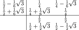
The Gauss–Legendre methods form a family of collocation methods based on Gauss quadrature. A Gauss–Legendre method with s stages has order 2s (thus, methods with arbitrarily high order can be constructed).^[17] The method with two stages (and thus order four) has Butcher tableau:

\begin{array}{c|cc} \frac12 - \frac16 \sqrt3 & \frac14 & \frac14 - \frac16 \sqrt3 \\ \frac12 + \frac16 \sqrt3 & \frac14 + \frac16 \sqrt3 & \frac14 \\ \hline & \frac12 & \frac12 \\ & \frac12+\frac12 \sqrt3 & \frac12-\frac12 \sqrt3 \end{array}

^[15]

Stability

The advantage of implicit Runge–Kutta methods over explicit ones is their greater stability, especially when applied to stiff equations. Consider the linear test equation y' = λy. A Runge–Kutta method applied to this equation reduces to the iteration $y_{n+1} = r(h\lambda) \, y_n$ , with r given by

r(z) = 1 + z b^T (I-zA)^{-1} e = \frac{\det(I-zA+zeb^T)}{\det(I-zA)},

^[18]

where e stands for the vector of ones. The function r is called the stability function.^[19] It follows from the formula that r is the quotient of two polynomials of degree s if the method has s stages. Explicit methods have a strictly lower triangular matrix A, which implies that det(I − zA) = 1 and that the stability function is a polynomial.^[20]

The numerical solution to the linear test equation decays to zero if | r(z) | < 1 with z = hλ. The set of such z is called the domain of absolute stability. In particular, the method is said to be A-stable if all z with Re(z) < 0 are in the domain of absolute stability. The stability function of an explicit Runge–Kutta method is a polynomial, so explicit Runge–Kutta methods can never be A-stable.^[20]

If the method has order p, then the stability function satisfies $r(z) = \textrm{e}^z + O(z^{p+1})$ as $z \to 0$ . Thus, it is of interest to study quotients of polynomials of given degrees that approximate the exponential function the best. These are known as Padé approximants. A Padé approximant with numerator of degree m and denominator of degree n is A-stable if and only if m ≤ n ≤ m + 2.^[21]

The Gauss–Legendre method with s stages has order 2s, so its stability function is the Padé approximant with m = n = s. It follows that the method is A-stable.^[22] This shows that A-stable Runge–Kutta can have arbitrarily high order. In contrast, the order of A-stable linear multistep methods cannot exceed two.^[23]

B-stability

The A-stability concept for the solution of differential equations is related to the linear autonomous equation $y'=\lambda y$ . Dahlquist proposed the investigation of stability of numerical schemes when applied to nonlinear systems that satisfy a monotonicity condition. The corresponding concepts were defined as G-stability for multistep methods (and the related one-leg methods) and B-stability (Butcher, 1975) for Runge–Kutta methods. A Runge–Kutta method applied to the non-linear system $y'=f(y)$ , which verifies $\langle f(y)-f(z),y-z \rangle<0$ , is called B-stable, if this condition implies $\|y_{n+1}-z_{n+1}\|\leq\|y_{n}-z_{n}\|$ for two numerical solutions.

Let $B$ , $M$ and $Q$ be three $s\times s$ matrices defined by

B=\operatorname{diag}(b_1,b_2,\ldots,b_s),\, M=BA+A^TB-bb^T,\, Q=BA^{-1}+A^{-T}B-A^{-T}bb^TA^{-1}.

A Runge–Kutta method is said to be algebraically stable ^[24] if the matrices $B$ and $M$ are both non-negative definite. A sufficient condition for B-stability ^[25] is: $B$ and $Q$ are non-negative definite.

Derivation of the Runge–Kutta fourth-order method

In general a Runge–Kutta method of order $s$ can be written as:

y_{t + h} = y_t + h \cdot \sum_{i=1}^s a_i k_i +\mathcal{O}(h^{s+1}),

where:

k_i = f\left(y_t + h \cdot \sum_{j = 1}^s \beta_{ij} k_j, t_n + \alpha_i h \right)

are increments obtained evaluating the derivatives of $y_t$ at the $i$ -th order.

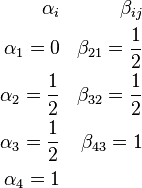
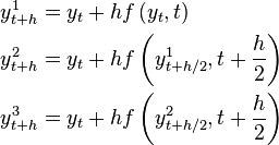
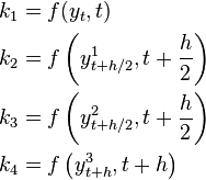
We develop the derivation^[26] for the Runge–Kutta fourth-order method using the general formula with $s=4$ evaluated, as explained above, at the starting point, the midpoint and the end point of any interval $(t, t +h)$ , thus we choose:

\begin{align} \alpha_i & & \beta_{ij} \\ \alpha_1 = 0 & &\beta_{21} = \frac{1}{2} \\ \alpha_2 = \frac{1}{2} & &\beta_{32} = \frac{1}{2} \\ \alpha_3 = \frac{1}{2} & &\beta_{43} = 1 \\ \alpha_4 = 1 & &\\ \end{align}

and $\beta_{ij} = 0$ otherwise. We begin by defining the following quantities:

\begin{align} y^1_{t+h} &= y_t + hf\left(y_t, t\right) \\ y^2_{t+h} &= y_t + hf\left(y^1_{t+h/2}, t+\frac{h}{2}\right) \\ y^3_{t+h} &= y_t + hf\left(y^2_{t+h/2}, t+\frac{h}{2}\right) \end{align}

where $y^1_{t+h/2} = \dfrac{y_t + y^1_{t+h}}{2}$ and $y^2_{t+h/2} = \dfrac{y_t + y^2_{t+h}}{2}$ If we define:

\begin{align} k_1 &= f(y_t, t) \\ k_2 &= f\left(y^1_{t+h/2}, t + \frac{h}{2}\right) \\ k_3 &= f\left(y^2_{t+h/2}, t + \frac{h}{2}\right) \\ k_4 &= f\left(y^3_{t+h}, t + h\right) \end{align}

and for the previous relations we can show that the following equalities holds up to $\mathcal{O}(h^2)$ :

\begin{align} k_2 &= f\left(y^1_{t+h/2}, t + \frac{h}{2}\right) = f\left(y_t + \frac{h}{2} k_1, t + \frac{h}{2}\right) \\ &= f\left(y_t, t\right) + \frac{h}{2} \frac{d}{dt}f\left(y_t,t\right) \\ k_3 &= f\left(y^2_{t+h/2}, t + \frac{h}{2}\right) = f\left(y_t + \frac{h}{2} f\left(y_t + \frac{h}{2} k_1, t + \frac{h}{2}\right), t + \frac{h}{2}\right) \\ &= f\left(y_t, t\right) + \frac{h}{2} \frac{d}{dt} \left[ f\left(y_t,t\right) + \frac{h}{2} \frac{d}{dt}f\left(y_t,t\right) \right] \\ k_4 &= f\left(y^3_{t+h}, t + h\right) = f\left(y_t + h f\left(y_t + \frac{h}{2} k_2, t + \frac{h}{2}\right), t + h\right) \\ &= f\left(y_t + h f\left(y_t + \frac{h}{2} f\left(y_t + \frac{h}{2} f\left(y_t, t\right), t + \frac{h}{2}\right), t + \frac{h}{2}\right), t + h\right) \\ &= f\left(y_t, t\right) + h \frac{d}{dt} \left[ f\left(y_t,t\right) + \frac{h}{2} \frac{d}{dt}\left[ f\left(y_t,t\right) + \frac{h}{2} \frac{d}{dt}f\left(y_t,t\right) \right]\right] \end{align}

where:

\frac{d}{dt} f(y_t, t) = \frac{\partial}{\partial y} f(y_t, t) \dot y_t + \frac{\partial}{\partial t} f(y_t, t) = f_y(y_t, t) \dot y + f_t(y_t, t) := \ddot y_t

is the total derivative of $f$ with respect to time.

If we now express the general formula using what we just derived we obtain:

\begin{align} y_{t+h} &= y_t + h \left\lbrace a \cdot f(y_t, t) + b \cdot \left[ f\left(y_t, t\right) + \frac{h}{2} \frac{d}{dt}f\left(y_t,t\right) \right] \right.+ \\ & {}+ c \cdot \left[ f\left(y_t, t\right) + \frac{h}{2} \frac{d}{dt} \left[ f\left(y_t,t\right) + \frac{h}{2} \frac{d}{dt}f\left(y_t,t\right) \right] \right] + \\ &{}+ d \cdot \left[f\left(y_t, t\right) + h \frac{d}{dt} \left[ f\left(y_t,t\right) + \frac{h}{2} \frac{d}{dt}\left[ f\left(y_t,t\right) + \left. \frac{h}{2} \frac{d}{dt}f\left(y_t,t\right) \right]\right]\right]\right\rbrace + \mathcal{O}(h^5) \\ &= y_t + a \cdot h f_t + b \cdot h f_t + b \cdot \frac{h^2}{2} \frac{df_t}{dt} + c \cdot h f_t+ c \cdot \frac{h^2}{2} \frac{df_t}{dt} + \\ &{}+ c \cdot \frac{h^3}{4} \frac{d^2f_t}{dt^2} + d \cdot h f_t + d \cdot h^2 \frac{df_t}{dt} + d \cdot \frac{h^3}{2} \frac{d^2f_t}{dt^2} + d \cdot \frac{h^4}{4} \frac{d^3f_t}{dt^3} + \mathcal{O}(h^5) \end{align}

and comparing this with the Taylor series of $y_{t+h}$ around $y_t$ :

\begin{align} y_{t+h} &= y_t + h \dot y_t + \frac{h^2}{2} \ddot y_t + \frac{h^3}{6} y^{(3)}_t + \frac{h^4}{24} y^{(4)}_t + \mathcal{O}(h^5) = \\ &= y_t + h f(y_t, t) + \frac{h^2}{2} \frac{d}{dt}f(y_t, t) + \frac{h^3}{6} \frac{d^2}{dt^2}f(y_t, t) + \frac{h^4}{24} \frac{d^3}{dt^3}f(y_t, t) \end{align}

we obtain a system of constraints on the coefficients:

\begin{cases} &a + b + c + d = 1 \\[6pt] & \frac{1}{2} b + \frac{1}{2} c + d = \frac{1}{2} \\[6pt] & \frac{1}{4} c + \frac{1}{2} d = \frac{1}{6} \\[6pt] & \frac{1}{4} d = \frac{1}{24} \end{cases}

which when solved gives $a = \frac{1}{6}, b = \frac{1}{3}, c = \frac{1}{3}, d = \frac{1}{6}$ as stated above.

Notes

↑ Press et al. 2007, p. 908; Süli & Mayers 2003, p. 328
1 2 Atkinson (1989, p. 423), Hairer, Nørsett & Wanner (1993, p. 134), Kaw & Kalu (2008, §8.4) and Stoer & Bulirsch (2002, p. 476) leave out the factor h in the definition of the stages. Ascher & Petzold (1998, p. 81), Butcher (2008, p. 93) and Iserles (1996, p. 38) use the y-values as stages.
1 2 Süli & Mayers 2003, p. 328
↑ Press et al. 2007, p. 907
↑ Iserles 1996, p. 38
↑ Iserles 1996, p. 39
↑ Butcher 2008, p. 187
↑ Butcher 2008, pp. 187–196
1 2 Süli & Mayers 2003, p. 352
↑ Hairer, Nørsett & Wanner (1993, p. 138) refer to Kutta (1901)
↑ Süli & Mayers 2003, p. 327
↑ Lambert 1991, p. 278
↑ Süli & Mayers 2003, pp. 349–351
↑ Iserles 1996, p. 41; Süli & Mayers 2003, pp. 351–352
1 2 Süli & Mayers 2003, p. 353
↑ Iserles 1996, pp. 43–44
↑ Iserles 1996, p. 47
↑ Hairer & Wanner 1996, pp. 40–41
↑ Hairer & Wanner 1996, p. 40
1 2 Iserles 1996, p. 60
↑ Iserles 1996, pp. 62–63
↑ Iserles 1996, p. 63
↑ This result is due to Dahlquist (1963).
↑ Lambert 1991, p. 275
↑ Lambert 1991, p. 274
↑ PDF reporting this derivation

References

Ascher, Uri M.; Petzold, Linda R. (1998), Computer Methods for Ordinary Differential Equations and Differential-Algebraic Equations, Philadelphia: Society for Industrial and Applied Mathematics, ISBN 978-0-89871-412-8 .
Atkinson, Kendall A. (1989), An Introduction to Numerical Analysis (2nd ed.), New York: John Wiley & Sons, ISBN 978-0-471-50023-0 .
Butcher, John C. (May 1963), Coefficients for the study of Runge-Kutta integration processes 3 (2), pp. 185–201, doi:10.1017/S1446788700027932 .
Butcher, John C. (1975), "A stability property of implicit Runge-Kutta methods", BIT 15: 358–361, doi:10.1007/bf01931672 .
Butcher, John C. (2008), Numerical Methods for Ordinary Differential Equations, New York: John Wiley & Sons, ISBN 978-0-470-72335-7 .
Cellier, F.; Kofman, E. (2006), Continuous System Simulation, Springer Verlag, ISBN 0-387-26102-8 .
Dahlquist, Germund (1963), "A special stability problem for linear multistep methods", BIT 3: 27–43, doi:10.1007/BF01963532, ISSN 0006-3835 .
Forsythe, George E.; Malcolm, Michael A.; Moler, Cleve B. (1977), Computer Methods for Mathematical Computations, Prentice-Hall (see Chapter 6).
Hairer, Ernst; Nørsett, Syvert Paul; Wanner, Gerhard (1993), Solving ordinary differential equations I: Nonstiff problems, Berlin, New York: Springer-Verlag, ISBN 978-3-540-56670-0 .
Hairer, Ernst; Wanner, Gerhard (1996), Solving ordinary differential equations II: Stiff and differential-algebraic problems (2nd ed.), Berlin, New York: Springer-Verlag, ISBN 978-3-540-60452-5 .
Iserles, Arieh (1996), A First Course in the Numerical Analysis of Differential Equations, Cambridge University Press, ISBN 978-0-521-55655-2 .
Lambert, J.D (1991), Numerical Methods for Ordinary Differential Systems. The Initial Value Problem, John Wiley & Sons, ISBN 0-471-92990-5
Kaw, Autar; Kalu, Egwu (2008), Numerical Methods with Applications (1st ed.), autarkaw.com .
Kutta, Martin Wilhelm (1901), "Beitrag zur näherungsweisen Integration totaler Differentialgleichungen", Zeitschrift für Mathematik und Physik 46: 435–453 .
Press, William H.; Flannery, Brian P.; Teukolsky, Saul A.; Vetterling, William T. (2007), "Section 17.1 Runge-Kutta Method", Numerical Recipes: The Art of Scientific Computing (3rd ed.), Cambridge University Press, ISBN 978-0-521-88068-8 . Also, Section 17.2. Adaptive Stepsize Control for Runge-Kutta.
Stoer, Josef; Bulirsch, Roland (2002), Introduction to Numerical Analysis (3rd ed.), Berlin, New York: Springer-Verlag, ISBN 978-0-387-95452-3 .
Süli, Endre; Mayers, David (2003), An Introduction to Numerical Analysis, Cambridge University Press, ISBN 0-521-00794-1 .
Tan, Delin; Chen, Zheng (2012), "On A General Formula of Fourth Order Runge-Kutta Method" (PDF), Journal of Mathematical Science & Mathematics Education 7.2: 1–10 .

External links

Hazewinkel, Michiel, ed. (2001), "Runge-Kutta method", Encyclopedia of Mathematics, Springer, ISBN 978-1-55608-010-4
On line calculator for Runge-Kutta methods by www.mathstools.com
Runge–Kutta 4th-Order Method
Runge Kutta Method for O.D.E.'s
DotNumerics: Ordinary Differential Equations for C# and VB.NET — Initial-value problem for nonstiff and stiff ordinary differential equations (explicit Runge–Kutta, implicit Runge–Kutta, Gear's BDF and Adams–Moulton).
GafferOnGames — A physics resource for computer programmers

Numerical methods for integration

First-order methods	Euler method Backward Euler Semi-implicit Euler Exponential Euler

Second-order methods	Verlet integration Velocity Verlet Trapezoidal rule Beeman's algorithm Midpoint method Heun's method Newmark-beta method Leapfrog integration

Higher-order methods	Exponential integrators Runge–Kutta methods List of Runge–Kutta methods Linear multistep method General linear methods Backward differentiation formula

This article is issued from Wikipedia - version of the Sunday, January 31, 2016. The text is available under the Creative Commons Attribution/Share Alike but additional terms may apply for the media files.