Polynomial regression
| Part of a series on Statistics |
| Regression analysis |
|---|
 |
| Models |
| Estimation |
| Background |
|
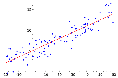
In statistics, polynomial regression is a form of linear regression in which the relationship between the independent variable x and the dependent variable y is modelled as an nth degree polynomial. Polynomial regression fits a nonlinear relationship between the value of x and the corresponding conditional mean of y, denoted E(y | x), and has been used to describe nonlinear phenomena such as the growth rate of tissues,[1] the distribution of carbon isotopes in lake sediments,[2] and the progression of disease epidemics.[3] Although polynomial regression fits a nonlinear model to the data, as a statistical estimation problem it is linear, in the sense that the regression function E(y | x) is linear in the unknown parameters that are estimated from the data. For this reason, polynomial regression is considered to be a special case of multiple linear regression.
The predictors resulting from the polynomial expansion of the "baseline" predictors are known as interaction features. Such predictors/features are also used in classification settings.[4]
History
Polynomial regression models are usually fit using the method of least squares. The least-squares method minimizes the variance of the unbiased estimators of the coefficients, under the conditions of the Gauss–Markov theorem. The least-squares method was published in 1805 by Legendre and in 1809 by Gauss. The first design of an experiment for polynomial regression appeared in an 1815 paper of Gergonne.[5][6] In the twentieth century, polynomial regression played an important role in the development of regression analysis, with a greater emphasis on issues of design and inference.[7] More recently, the use of polynomial models has been complemented by other methods, with non-polynomial models having advantages for some classes of problems.
Definition and example

The goal of regression analysis is to model the expected value of a dependent variable y in terms of the value of an independent variable (or vector of independent variables) x. In simple linear regression, the model
is used, where ε is an unobserved random error with mean zero conditioned on a scalar variable x. In this model, for each unit increase in the value of x, the conditional expectation of y increases by a1 units.
In many settings, such a linear relationship may not hold. For example, if we are modeling the yield of a chemical synthesis in terms of the temperature at which the synthesis takes place, we may find that the yield improves by increasing amounts for each unit increase in temperature. In this case, we might propose a quadratic model of the form
In this model, when the temperature is increased from x to x + 1 units, the expected yield changes by a1 + 2a2x. The fact that the change in yield depends on x is what makes the relationship nonlinear (this must not be confused with saying that this is nonlinear regression; on the contrary, this is still a case of linear regression).
In general, we can model the expected value of y as an nth degree polynomial, yielding the general polynomial regression model
Conveniently, these models are all linear from the point of view of estimation, since the regression function is linear in terms of the unknown parameters a0, a1, .... Therefore, for least squares analysis, the computational and inferential problems of polynomial regression can be completely addressed using the techniques of multiple regression. This is done by treating x, x2, ... as being distinct independent variables in a multiple regression model.
Matrix form and calculation of estimates
The polynomial regression model
can be expressed in matrix form in terms of a design matrix  , a response vector
  , a parameter vector
  , and a vector
  of random errors. The ith row of
  and
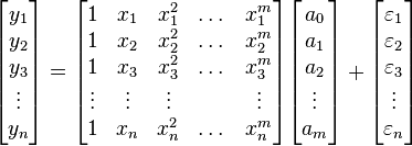
and  will contain the x and y value for the ith data sample. Then the model can be written as a system of linear equations:
which when using pure matrix notation is written as
The vector of estimated polynomial regression coefficients (using ordinary least squares estimation) is
This is the unique least squares solution as long as  has linearly independent columns. Since
  is a Vandermonde matrix, this is guaranteed to hold provided that at least m + 1 of the xi are distinct (for which m < n is a necessary condition).
Interpretation
Although polynomial regression is technically a special case of multiple linear regression, the interpretation of a fitted polynomial regression model requires a somewhat different perspective. It is often difficult to interpret the individual coefficients in a polynomial regression fit, since the underlying monomials can be highly correlated. For example, x and x2 have correlation around 0.97 when x is uniformly distributed on the interval (0, 1). Although the correlation can be reduced by using orthogonal polynomials, it is generally more informative to consider the fitted regression function as a whole. Point-wise or simultaneous confidence bands can then be used to provide a sense of the uncertainty in the estimate of the regression function.
Alternative approaches
Polynomial regression is one example of regression analysis using basis functions to model a functional relationship between two quantities. More specifically, it replaces  in linear regression with polynomial basis
  ,e.g.
,e.g. ![[1,x] \stackrel{\phi}{\rightarrow} [1,x,x^2,...,x^d]](../I/m/d0324fbbba5c7a1c011e362c8496bfa1.png) . A drawback of polynomial bases is that the basis functions are "non-local", meaning that the fitted value of y at a given value x = x0 depends strongly on data values with x far from x0.[8] In modern statistics, polynomial basis-functions are used along with new basis functions, such as splines, radial basis functions, and wavelets. These families of basis functions offer a more parsimonious fit for many types of data.
. A drawback of polynomial bases is that the basis functions are "non-local", meaning that the fitted value of y at a given value x = x0 depends strongly on data values with x far from x0.[8] In modern statistics, polynomial basis-functions are used along with new basis functions, such as splines, radial basis functions, and wavelets. These families of basis functions offer a more parsimonious fit for many types of data.
The goal of polynomial regression is to model a non-linear relationship between the independent and dependent variables (technically, between the independent variable and the conditional mean of the dependent variable). This is similar to the goal of nonparametric regression, which aims to capture non-linear regression relationships. Therefore, non-parametric regression approaches such as smoothing can be useful alternatives to polynomial regression. Some of these methods make use of a localized form of classical polynomial regression.[9] An advantage of traditional polynomial regression is that the inferential framework of multiple regression can be used (this also holds when using other families of basis functions such as splines).
A final alternative is to use kernelized models such as support vector regression with a polynomial kernel.
See also
- Curve fitting
- Response surface methodology
- Line regression
- Polynomial and rational function modeling
- Polynomial interpolation
Notes
- Microsoft Excel makes use of polynomial regression when fitting a trendline to data points on an X Y scatter plot.[10]
References
- ↑ Shaw, P; et al. (2006). "Intellectual ability and cortical development in children and adolescents". Nature 440 (7084): 676–679. doi:10.1038/nature04513. PMID 16572172.
- ↑ Barker, PA; Street-Perrott, FA; Leng, MJ; Greenwood, PB; Swain, DL; Perrott, RA; Telford, RJ; Ficken, KJ (2001). "A 14,000-Year Oxygen Isotope Record from Diatom Silica in Two Alpine Lakes on Mt. Kenya". Science 292 (5525): 2307–2310. doi:10.1126/science.1059612. PMID 11423656.
- ↑ Greenland, Sander (1995). "Dose-Response and Trend Analysis in Epidemiology: Alternatives to Categorical Analysis". Epidemiology (Lippincott Williams & Wilkins) 6 (4): 356–365. doi:10.1097/00001648-199507000-00005. JSTOR 3702080. PMID 7548341.
- ↑ Yin-Wen Chang; Cho-Jui Hsieh; Kai-Wei Chang; Michael Ringgaard; Chih-Jen Lin (2010). "Training and testing low-degree polynomial data mappings via linear SVM". Journal of Machine Learning Research 11: 1471–1490.
- ↑ Gergonne, J. D. (November 1974) [1815]. "The application of the method of least squares to the interpolation of sequences". Historia Mathematica (Translated by Ralph St. John and S. M. Stigler from the 1815 French ed.) 1 (4): 439–447. doi:10.1016/0315-0860(74)90034-2.
- ↑ Stigler, Stephen M. (November 1974). "Gergonne's 1815 paper on the design and analysis of polynomial regression experiments". Historia Mathematica 1 (4): 431–439. doi:10.1016/0315-0860(74)90033-0.
- ↑ Smith, Kirstine (1918). "On the Standard Deviations of Adjusted and Interpolated Values of an Observed Polynomial Function and its Constants and the Guidance They Give Towards a Proper Choice of the Distribution of the Observations". Biometrika 12 (1/2): 1–85. doi:10.2307/2331929. JSTOR 2331929. External link in
|journal=(help) - ↑ Such "non-local" behavior is a property of analytic functions that are not constant (everywhere). Such "non-local" behavior has been widely discussed in statistics:
- Magee, Lonnie (1998). "Nonlocal Behavior in Polynomial Regressions". The American Statistician (American Statistical Association) 52 (1): 20–22. doi:10.2307/2685560. JSTOR 2685560.
- ↑ Fan, Jianqing (1996). "Local Polynomial Modelling and Its Applications". Monographs on Statistics and Applied Probability. Chapman & Hall/CRC. ISBN 0-412-98321-4.
|chapter=ignored (help) - ↑ [Tutorial: Data Analysis with Excel https://facultystaff.richmond.edu/~cstevens/301/Excel4.html]
| ||||||||||||||||||||||||||||||||||||||||||||||||||||||||||||||||||||||||||||||||||||||||||||||||||||||||||||||||||||||||||||||||||||||||||||||||||||||||||||||||||||||||||||||||||||||||||||||||||||||||||||||||||||||||||||||||
| ||||||||||||||||||||||||||||||||||||||||||||||||||||||||||||


