Parameterized post-Newtonian formalism
| General relativity | ||||||
|---|---|---|---|---|---|---|
  | ||||||
|
Fundamental concepts |
||||||
|
||||||
Post-Newtonian formalism is a calculational tool that expresses Einstein's (nonlinear) equations of gravity in terms of the lowest-order deviations from Newton's law of universal gravitation. This allows approximations to Einstein's equations to be made in the case of weak fields. Higher order terms can be added to increase accuracy, but for strong fields sometimes it is preferable to solve the complete equations numerically. Some of these post-Newtonian approximations are expansions in a small parameter, which is the ratio of the velocity of the matter forming the gravitational field to the speed of light, which in this case is better called the speed of gravity. In the limit, when the fundamental speed of gravity becomes infinite, the post-Newtonian expansion reduces to Newton's law of gravity.
The parameterized post-Newtonian formalism or PPN formalism is a version of this formulation that explicitly details the parameters in which a general theory of gravity can differ from Newtonian gravity. It is used as a tool to compare Newtonian and Einsteinian gravity in the limit in which the gravitational field is weak and generated by objects moving slowly compared to the speed of light. In general, PPN formalism can be applied to all metric theories of gravitation in which all bodies satisfy the Einstein equivalence principle (EEP). The speed of light remains constant in PPN formalism and it assumes that the metric tensor is always symmetric.
History
The earliest parameterizations of the post-Newtonian approximation were performed by Sir Arthur Stanley Eddington in 1922. However, they dealt solely with the vacuum gravitational field outside an isolated spherical body. Dr. Ken Nordtvedt (1968, 1969) expanded this to include 7 parameters. Clifford Martin Will (1971) introduced a stressed, continuous matter description of celestial bodies.
The versions described here are based on Wei-Tou Ni (1972), Will and Nordtvedt (1972), Charles W. Misner et al. (1973) (see Gravitation (book)), and Will (1981, 1993) and have 10 parameters.
Beta-delta notation
Ten post-Newtonian parameters completely characterize the weak-field behavior of the theory. The formalism has been a valuable tool in tests of general relativity. In the notation of Will (1971), Ni (1972) and Misner et al. (1973) they have the following values:
 | How much space curvature  is produced by unit rest mass ? is produced by unit rest mass ? |
 | How much nonlinearity is there in the superposition law for gravity  ? ? |
 | How much gravity is produced by unit kinetic energy  ? ? |
 | How much gravity is produced by unit gravitational potential energy  ? ? |
 | How much gravity is produced by unit internal energy  ? ? |
 | How much gravity is produced by unit pressure  ? ? |
 | Difference between radial and transverse kinetic energy on gravity |
 | Difference between radial and transverse stress on gravity |
 | How much dragging of inertial frames  is produced by unit momentum is produced by unit momentum  ? ? |
 | Difference between radial and transverse momentum on dragging of inertial frames |
 is the 4 by 4 symmetric metric tensor and indexes
  and
and  go from 1 to 3.
In Einstein's theory, the values of these parameters are chosen (1) to fit Newton's Law of gravity in the limit of velocities and mass approaching zero, (2) to ensure conservation of energy, mass, momentum, and angular momentum, and (3) to make the equations independent of the reference frame. In this notation, general relativity has PPN parameters
 and
and 
Alpha-zeta notation
In the more recent notation of Will & Nordtvedt (1972) and Will (1981, 1993, 2006) a different set of ten PPN parameters is used.


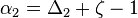


 is calculated from
The meaning of these is that  ,
,  and
and  measure the extent of preferred frame effects.
  ,
,  ,
,  ,
,  and measure the failure of conservation of energy, momentum and angular momentum.
In this notation, general relativity has PPN parameters
 and
and 
The mathematical relationship between the metric, metric potentials and PPN parameters for this notation is:


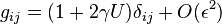
where repeated indexes are summed.  is on the order of potentials such as
  , the square magnitude of the coordinate velocities of matter, etc.
  is the velocity vector of the PPN coordinate system relative to the mean rest-frame of the universe.
  is the square magnitude of that velocity.
  if and only if
  ,
,  otherwise.
There are ten metric potentials, ,  ,
,  ,
,  ,
,  ,
,  ,
,  ,
,  ,
,  and
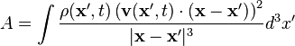
and  , one for each PPN parameter to ensure a unique solution. 10 linear equations in 10 unknowns are solved by inverting a 10 by 10 matrix. These metric potentials have forms such as:
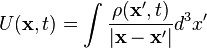
which is simply another way of writing the Newtonian gravitational potential,


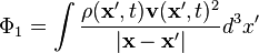

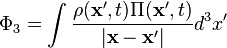

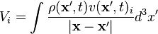
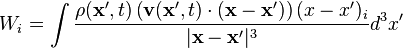
where  is the density of rest mass,
  is the internal energy per unit rest mass, is the pressure as measured in a local freely falling frame momentarily comoving with the matter, and
  is the coordinate velocity of the matter.
Stress-energy tensor for a perfect fluid takes form


How to apply PPN
Examples of the process of applying PPN formalism to alternative theories of gravity can be found in Will (1981, 1993). It is a nine step process:
- Step 1: Identify the variables, which may include: (a) dynamical gravitational variables such as the metric
 , scalar field
  , vector field
  , tensor field
  and so on; (b) prior-geometrical variables such as a flat background metric
  , cosmic time function
  , and so on; (c) matter and non-gravitational field variables.
- Step 2: Set the cosmological boundary conditions. Assume a homogeneous isotropic cosmology, with isotropic coordinates in the rest frame of the universe. A complete cosmological solution may or may not be needed. Call the results
 ,
,  ,
,  ,
,  .
.
- Step 3: Get new variables from
 , with
  ,
,  or
or  if needed.
- Step 4: Substitute these forms into the field equations, keeping only such terms as are necessary to obtain a final consistent solution for
 . Substitute the perfect fluid stress tensor for the matter sources.
- Step 5: Solve for
 to
to  . Assuming this tends to zero far from the system, one obtains the form
  where
where  is the Newtonian gravitational potential and
  may be a complicated function including the gravitational "constant"
  . The Newtonian metric has the form
  ,
,  ,
,  . Work in units where the gravitational "constant" measured today far from gravitating matter is unity so set
  .
.
- Step 6: From linearized versions of the field equations solve for
 to and
  to
to  .
.
- Step 7: Solve for to
 . This is the messiest step, involving all the nonlinearities in the field equations. The stress–energy tensor must also be expanded to sufficient order.
- Step 8: Convert to local quasi-Cartesian coordinates and to standard PPN gauge.
- Step 9: By comparing the result for with the equations presented in PPN with alpha-zeta parameters, read off the PPN parameter values.
Comparisons between theories of gravity
A table comparing PPN parameters for 23 theories of gravity can be found in Alternatives to general relativity#PPN parameters for a range of theories.
Most metric theories of gravity can be lumped into categories. Scalar theories of gravitation include conformally flat theories and stratified theories with time-orthogonal space slices.
In conformally flat theories such as Nordström's theory of gravitation the metric is given by  and for this metric
  , which violently disagrees with observations. In stratified theories such as Yilmaz theory of gravitation the metric is given by
 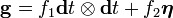 and for this metric
 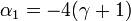 , which also disagrees violently with observations.
Another class of theories is the quasilinear theories such as Whitehead's theory of gravitation. For these  . The relative magnitudes of the harmonics of the Earth's tides depend on and , and measurements show that quasilinear theories disagree with observations of Earth's tides.
Another class of metric theories is the bimetric theory. For all of these  is non-zero. From the precession of the solar spin we know that
  , and that effectively rules out bimetric theories.
Another class of metric theories is the scalar tensor theories, such as Brans–Dicke theory. For all of these,  . The limit of
  means that
  would have to be very large, so these theories are looking less and less likely as experimental accuracy improves.
The final main class of metric theories is the vector-tensor theories. For all of these the gravitational "constant" varies with time and is non-zero. Lunar laser ranging experiments tightly constrain the variation of the gravitational "constant" with time and , so these theories are also looking unlikely.
There are some metric theories of gravity that do not fit into the above categories, but they have similar problems.
Accuracy from experimental tests
Bounds on the PPN parameters Will (2006)
| Parameter | Bound | Effects | Experiment |
|---|---|---|---|
 |  x x  | Time delay, Light deflection | Cassini tracking |
 |  x x  | Perihelion shift | Perihelion shift |
| | x  | Nordtvedt effect with assumption 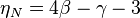 | Nordtvedt effect |
| |  | Earth tides | Gravimeter data |
| | | Orbit polarization | Lunar laser ranging |
| |  x x  | Spin precession | Sun axis' alignment with ecliptic |
| | x  | Self-acceleration | Pulsar spin-down statistics |
 |  x x | Nordtvedt effect | Lunar Laser Ranging |
| |  | - | Combined PPN bounds |
| | x † | Binary pulsar acceleration | PSR 1913+16 |
| |  | Newton's 3rd law | Lunar acceleration |
| |  ‡ ‡ | - | Kreuzer experiment |
† Will, C.M., Is momentum conserved? A test in the binary system PSR 1913 + 16, Astrophysical Journal, Part 2 - Letters (ISSN 0004-637X), vol. 393, no. 2, July 10, 1992, p. L59-L61.
‡ Based on  from Will (1976, 2006). It is theoretically possible for an alternative model of gravity to bypass this bound, in which case the bound is
  from Ni (1972).
References
- Eddington, A. S. (1922) The Mathematical Theory of Relativity, Cambridge University Press.
- Misner, C. W., Thorne, K. S. & Wheeler, J. A. (1973) Gravitation, W. H. Freeman and Co.
- Nordtvedt Jr, K. (1968) Equivalence principle for massive bodies II: Theory, Phys. Rev. 169, 1017-1025.
- Nordtvedt Jr, K. (1969) Equivalence principle for massive bodies including rotational energy and radiation pressure, Phys. Rev. 180, 1293-1298.
- Will, C. M. (1971) Theoretical frameworks for testing relativistic gravity II: Parameterized post-Newtonian hydrodynamics and the Nordtvedt effect, Astrophys. J. 163, 611-628.
- Will, C. M. (1976) Active mass in relativistic gravity: Theoretical interpretation of the Kreuzer experiment, Astrophys. J., 204, 224-234.
- Will, C. M. (1981, 1993) Theory and Experiment in Gravitational Physics, Cambridge University Press. ISBN 0-521-43973-6.
- Will, C. M., (2006) The Confrontation between General Relativity and Experiment, http://relativity.livingreviews.org/Articles/lrr-2006-3/
- Will, C. M., and Nordtvedt Jr., K (1972) Conservation laws and preferred frames in relativistic gravity I, The Astrophysical Journal 177, 757.
See also
- Alternatives to general relativity#PPN parameters for a range of theories
- Linearized gravity
- Peskin-Takeuchi parameter The same thing as PPN, but for electroweak theory instead of gravitation
- Tests of general relativity
| ||||||||||||||||||||||||||||||||||||||||||
| ||||||||||||||||||||||||||||||||||||||||||||||||||||||||