Objectivity (frame invariance)
The concept of objectivity in science means that qualitative and quantitative descriptions of physical phenomena remain unchanged when the phenomena are observed under a variety of conditions. For example, physical processes (e.g. material properties) are invariant under changes of observers; that is, it is possible to reconcile observations of the process into a single coherent description of it.
Euclidean transformation
Physical processes can be described by an observer denoted by  . In Euclidean three-dimensional space and time, an observer can measure relative positions of points in space and intervals of time.
Consider an event in Euclidean space characterized by the pairs  and
and  where
where  is a position vector and
  is a scalar representing time. This pair is mapped to another one denoted by the
  superscript. This mapping is done with the orthogonal time-dependent second order tensor
  in a way such that the distance between the pairs is kept the same. Therefore one can write:
By introducing a vector  and a real number
  denoting the time shift, the relationship between
  and
and  can be expressed
The one-to-one mapping connection of the pair  with its corresponding pair
  is referred to as a Euclidean transformation.
Displacement
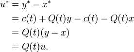
A physical quantity like displacement should be invariant relative to a change of observer. Consider one event recorded by two observers; for  , point
  moves to position
  whereas for
  , the same point
  moves to
  . For
. For  , the displacement is
  . On the other hand, for
  , one can write:
Any spatial vector field  that transforms such that:
is said to be objective, since  .
.
Velocity
Because  is a rotation matrix,
  where
where  is the identity matrix. Using this relation, the inverse of the Euclidean transformation can be written as:
The velocity can be obtained by differentiating the above expression:
By reorganizing the terms in the above equation, one can obtain:
where
is a skew tensor representing the spin of the reference frame of observer  relative to the reference frame of observer
  (Holzapfel 2000). To simplify the mathematical notation, the arguments of functions will no longer be written.
From the above expression, one can conclude that velocity is not objective because of the presence of the extra terms  and
and ![\Omega[x^*-c]](../I/m/9bf94eacd73742fcf7585a04361024a1.png) . Nevertheless, the velocity field can be made objective by constraining the change of observer to:
. Nevertheless, the velocity field can be made objective by constraining the change of observer to:
A time-independent rigid transformation such as:
respects this condition.
Acceleration
The material time derivative of the spatial velocity  returns the spatial acceleration
  . By differentiating the transformation law for the spatial velocity, one can obtain:
which can be rewritten as the following:
Just like the spatial velocity, the acceleration is not an objective quantity for a general change of observer (Holzapfel 2000). As for the spatial velocity, the acceleration can also be made objective by constraining the change of observer. One possibility would be to use the time-independent rigid transformation introduced above.
Objectivity for higher-order tensor fields
A tensor field of order  and denoted
  is objective if, during a general change of observer, the transformation is given by:
Example for a second-order tensor
Introducing a second order tensor  , one can find with the above definition of objectivity that:
Example for a scalar field
The general condition of objectivity for a tensor of order  can be applied to a scalar field
  for which
  . The transformation would give:
Physically, this means that a scalar field is independent of the observer. Temperature is an example of scalar field and it is easy to understand that the temperature at a given point in a room and at a given time would have the same value for any observer.
Euclidean transformation of others kinematic quantities
Deformation gradient
The deformation gradient at point  and at its associated point
  is a second order tensor given by:
where  represents the material coordinates. Using the chain rule, one can write:
From the above equation, one can conclude that the deformation gradient  is objective even though it transforms like a vector and not like a second order tensor. This is because one index of the tensor describes the material coordinates
  which are independent of the observer (Holzapfel 2000).
Cauchy stress tensor
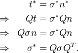
The Cauchy traction vector  is related to the Cauchy stress tensor
  at a given point
  by the outward normal to the surface
  such that:
  . The Cauchy traction vector for another observer can be simply written as
  , where
  and
and  are both objective vectors. Knowing that, one can write:
This demonstrates that the Cauchy stress tensor is objective.
Piola–Kirchhoff stress tensors
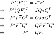
The first Piola–Kirchhoff stress tensor  is defined as:
where  . It is also interesting to know that since
  is a rotation matrix:
Using identities developed previously, one can write:
This proves that the first Piola–Kirchhoff stress tensor is objective. Similarly to the deformation gradient, this second order tensor transforms like a vector.
The second Piola–Kirchhoff stress tensor  is also objective and transforms like a scalar field. This can be easily demonstrated:
The three stress tensors,  ,
,  and
and  , studied here were all found to be objective. Therefore, they are all suitable to describe the material response and develop constitutive laws, since they are independent of the observer.
Objective rates
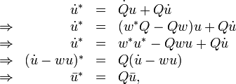
It was shown above that even if a displacement field is objective, the velocity field is not. An objective vector  and an objective tensor
  usually do not conserve their objectivity through time differentiation as demonstrated below:
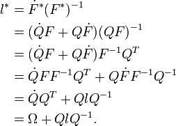
Objectivity rates are modified material derivatives that allows to have an objective time differentiation. Before presenting some examples of objectivity rates, certain other quantities need to be introduced. First, the spatial velocity gradient  is defined as:
where  is a symmetric tensor and
  is a skew tensor called the spin tensor. For a given
  ,
,  and
and  are uniquely defined. The Euclidean transformation for the spatial velocity gradient can be written as:
Substituting  in the above equation, one can obtain two following relations:
Substituting the above result in the previously obtained equation for the rate of an objective vector, one can write:
where the co-rotational rate of the objective vector field  is defined as:
and represents an objective quantity. Similarly, using the above equations, one can obtain the co-rotational rate of the objective second-order tensor field  :
:
This co-rotational rate second order tensor is defined as:
This objective rate is known as the Jaumann–Zaremba rate and it is often used in plasticity theory. Many different objective rates can be developed. Objective stress rates are of particular interest in continuum mechanics because they are required for constitutive models, expressed in terms of time derivatives of stress and strain, to be frame-indifferent.
Invariance of material response
The principal of material invariance basically means that the material properties are independent of the observer. In this section it will be shown how this principle adds constraints to constitutive laws.
Cauchy-elastic materials
A Cauchy-elastic material depends only on the current state of deformation at a given time (Holzapfel 2000). In other words, the material is independent of the deformation path and time.
Neglecting the effect of temperature and assuming the body to be homogeneous, a constitutive equation for the Cauchy stress tensor can be formulated based on the deformation gradient:
This constitutive equation for another arbitrary observer can be written  . Knowing that the Cauchy stress tensor
  and the deformation gradient
  are objective quantities, one can write:
The above is a condition that the constitutive law  has to respect to make sure that the response of the material will be independent of the observer. Similar conditions can be derived for constitutive laws relating the deformation gradient to the first or second Piola–Kirchhoff stress tensor.
Isotropic Cauchy-elastic materials
Here, it will be assumed that the Cauchy stress tensor  is a function of the left Cauchy–Green tensor
  . The constitutive equation may be written:
In order to find the restriction on  which will ensure the principle of material frame-indifference, one can write:
A constitutive equation that respects the above condition is said to be isotropic (Holzapfel 2000). Physically, this characteristic means that the material has no preferential direction. Wood and most fibre-reinforced composites are generally stronger in the direction of their fibres therefore they are not isotropic materials (they are qualified as anisotropic).
See also
- Cartesian coordinate system
- Finite strain theory
- Lagrangian and Eulerian coordinates
- Piola–Kirchhoff stress tensor
- Stress (physics)
- Cauchy stress tensor
- Principle of material objectivity
- Objective stress rate
- Hypoelastic material
References
- Cirak, F. (2007). Lecture Notes 5R14: Nonlinear Solid Mechanics. Department of Engineering, University of Cambridge.
- Gurtin, M.E. (1981). An Introduction to Continuum Mechanics. Academic Press. ISBN 978-0-12-309750-7.
- Holzapfel, G.A. (2000). Nonlinear Solid Mechanics: A Continuum Approach for Engineering. Wiley. ISBN 978-0-471-82319-3.
- Leigh, D.C. (1968). Nonlinear Continuum Mechanics. McGraw-Hill. ISBN 978-0-07-037085-2.
- Martinec, A. "Lecture Notes: Continuum Mechanics, Chapter 5: Objectivity" (PDF). Department of Geophysics, Charles University, Prague.



![\ x = Q(t)^T[x^*-c(t)].](../I/m/eca71fe71fa39031e6c60c68e16da40b.png)
![\ v(x,t) = \dot{x} = \dot{Q}(t)^T[x^*-c(t)] + Q(t)^T[v^*-\dot{c}(t)].](../I/m/37303b793b00f87e113d9d8fa13d81db.png)
![\ \begin{align} v^*(x^*,t) & = Q(t)v + \dot{c}(t) - Q(t)\dot{Q}(t)^T[x^*-c(t)]\\
& = Q(t)v + \dot{c}(t) + \Omega(t)[x^*-c(t)], \end{align}](../I/m/28d15630d686ef823da143dc9e299258.png)


