Exponential family
- "Natural parameter" links here. For the usage of this term in differential geometry, see differential geometry of curves.
In probability and statistics, an exponential family is a set of probability distributions of a certain form, specified below. This special form is chosen for mathematical convenience, on account of some useful algebraic properties, as well as for generality, as exponential families are in a sense very natural sets of distributions to consider. The concept of exponential families is credited to[1] E. J. G. Pitman,[2] G. Darmois,[3] and B. O. Koopman[4] in 1935–36. The term exponential class is sometimes used in place of "exponential family".[5]
The exponential families include many of the most common distributions, including the normal, exponential, gamma, chi-squared, beta, Dirichlet, Bernoulli, categorical, Poisson, Wishart, Inverse Wishart and many others. A number of common distributions are exponential families only when certain parameters are considered fixed and known, e.g. binomial (with fixed number of trials), multinomial (with fixed number of trials), and negative binomial (with fixed number of failures). Examples of common distributions that are not exponential families are Student's t, most mixture distributions, and even the family of uniform distributions with unknown bounds. See the section below on examples for more discussion.
Consideration of exponential-family distributions provides a general framework for selecting a possible alternative parameterisation of the distribution, in terms of natural parameters, and for defining useful sample statistics, called the natural sufficient statistics of the family. For more information, see below.
Definition
The following is a sequence of increasingly more general definitions of an exponential family. A casual reader may wish to restrict attention to the first and simplest definition, which corresponds to a single-parameter family of discrete or continuous probability distributions.
Scalar parameter
A single-parameter exponential family is a set of probability distributions whose probability density function (or probability mass function, for the case of a discrete distribution) can be expressed in the form
where T(x), h(x), η(θ), and A(θ) are known functions.
An alternative, equivalent form often given is
or equivalently
The value θ is called the parameter of the family.
Note that x is often a vector of measurements, in which case T(x) may be a function from the space of possible values of x to the real numbers. More generally, η(θ) and T(x) can each be vector-valued such that  is real-valued.
If η(θ) = θ, then the exponential family is said to be in canonical form. By defining a transformed parameter η = η(θ), it is always possible to convert an exponential family to canonical form. The canonical form is non-unique, since η(θ) can be multiplied by any nonzero constant, provided that T(x) is multiplied by that constant's reciprocal, or a constant c can be added to η(θ) and h(x) multiplied by  to offset it.
Even when x is a scalar, and there is only a single parameter, the functions η(θ) and T(x) can still be vectors, as described below.
Note also that the function A(θ) or equivalently g(θ) is automatically determined once the other functions have been chosen, and assumes a form that causes the distribution to be normalized (sum or integrate to one over the entire domain). Furthermore, both of these functions can always be written as functions of η, even when η(θ) is not a one-to-one function, i.e. two or more different values of θ map to the same value of η(θ), and hence η(θ) cannot be inverted. In such a case, all values of θ mapping to the same η(θ) will also have the same value for A(θ) and g(θ).
Further down the page is the example of a normal distribution with unknown mean and known variance.
Factorization of the variables involved
What is important to note, and what characterizes all exponential family variants, is that the parameter(s) and the observation variable(s) must factorize (can be separated into products each of which involves only one type of variable), either directly or within either part (the base or exponent) of an exponentiation operation. Generally, this means that all of the factors constituting the density or mass function must be of one of the following forms:
where f and h are arbitrary functions of x; g and j are arbitrary functions of θ; and c is an arbitrary "constant" expression (i.e. an expression not involving x or θ).
There are further restrictions on how many such factors can occur. For example, the two expressions:
are the same, i.e. a product of two "allowed" factors. However, when rewritten into the factorized form,
it can be seen that it cannot be expressed in the required form. (However, a form of this sort is a member of a curved exponential family, which allows multiple factorized terms in the exponent.)
To see why an expression of the form
qualifies, note that
and hence factorizes inside of the exponent. Similarly,
and again factorizes inside of the exponent.
Note also that a factor consisting of a sum where both types of variables are involved (e.g. a factor of the form  ) cannot be factorized in this fashion (except in some cases where occurring directly in an exponent); this is why, for example, the Cauchy distribution and Student's t distribution are not exponential families.
Vector parameter
The definition in terms of one real-number parameter can be extended to one real-vector parameter
A family of distributions is said to belong to a vector exponential family if the probability density function (or probability mass function, for discrete distributions) can be written as
Or in a more compact form,
This form writes the sum as a dot product of vector-valued functions  and
and  .
.
An alternative, equivalent form often seen is
As in the scalar valued case, the exponential family is said to be in canonical form if
A vector exponential family is said to be curved if the dimension of
is less than the dimension of the vector
That is, if the dimension of the parameter vector is less than the number of functions of the parameter vector in the above representation of the probability density function. Note that most common distributions in the exponential family are not curved, and many algorithms designed to work with any member of the exponential family implicitly or explicitly assume that the distribution is not curved.
Note that, as in the above case of a scalar-valued parameter, the function  or equivalently
  is automatically determined once the other functions have been chosen, so that the entire distribution is normalized. In addition, as above, both of these functions can always be written as functions of
  , regardless of the form of the transformation that generates
  from
from  . Hence an exponential family in its "natural form" (parametrized by its natural parameter) looks like
or equivalently
Note that the above forms may sometimes be seen with  in place of
  . These are exactly equivalent formulations, merely using different notation for the dot product.
Further down the page is the example of a normal distribution with unknown mean and variance.
Vector parameter, vector variable
The vector-parameter form over a single scalar-valued random variable can be trivially expanded to cover a joint distribution over a vector of random variables. The resulting distribution is simply the same as the above distribution for a scalar-valued random variable with each occurrence of the scalar x replaced by the vector
Note that the dimension k of the random variable need not match the dimension d of the parameter vector, nor (in the case of a curved exponential function) the dimension s of the natural parameter  and sufficient statistic T(x).
The distribution in this case is written as
Or more compactly as
Or alternatively as
Measure-theoretic formulation
We use cumulative distribution functions (cdf) in order to encompass both discrete and continuous distributions.
Suppose H is a non-decreasing function of a real variable. Then Lebesgue–Stieltjes integrals with respect to dH(x) are integrals with respect to the "reference measure" of the exponential family generated by H.
Any member of that exponential family has cumulative distribution function
If F is a continuous distribution with a density, one can write dF(x) = f(x) dx.
H(x) is a Lebesgue–Stieltjes integrator for the reference measure. When the reference measure is finite, it can be normalized and H is actually the cumulative distribution function of a probability distribution. If F is absolutely continuous with a density, then so is H, which can then be written dH(x) = h(x) dx. If F is discrete, then H is a step function (with steps on the support of F).
Interpretation
In the definitions above, the functions T(x), η(θ) and A(η) were apparently arbitrarily defined. However, these functions play a significant role in the resulting probability distribution.
- T(x) is a sufficient statistic of the distribution. For exponential families, the sufficient statistic is a function of the data that fully summarizes the data x within the density function. This means that, for any data sets x and y, the density value is the same if T(x) = T(y). This is true even if x and y are quite different—that is,
 . The dimension of T(x) equals the number of parameters of θ and encompasses all of the information regarding the data related to the parameter θ. The sufficient statistic of a set of independent identically distributed data observations is simply the sum of individual sufficient statistics, and encapsulates all the information needed to describe the posterior distribution of the parameters, given the data (and hence to derive any desired estimate of the parameters). This important property is further discussed below.
- η is called the natural parameter. The set of values of η for which the function
 is finite is called the natural parameter space. It can be shown that the natural parameter space is always convex.
- A(η) is called the log-partition function because it is the logarithm of a normalization factor, without which
 would not be a probability distribution ("partition function" is often used in statistics as a synonym of "normalization factor"):
The function A is important in its own right, because the mean, variance and other moments of the sufficient statistic T(x) can be derived simply by differentiating A(η). For example, because ln(x) is one of the components of the sufficient statistic of the gamma distribution, ![\mathbb{E}[\ln x]](../I/m/8c39935fcc4a67dde30aa15a7e3ee741.png) can be easily determined for this distribution using A(η). Technically, this is true because
can be easily determined for this distribution using A(η). Technically, this is true because
is the cumulant generating function of the sufficient statistic.
Properties
Exponential families have a large number of properties that make them extremely useful for statistical analysis. In many cases, it can be shown that, except in a few exceptional cases, only exponential families have these properties. Examples:
- Exponential families have sufficient statistics that can summarize arbitrary amounts of independent identically distributed data using a fixed number of values.
- Exponential families have conjugate priors, an important property in Bayesian statistics.
- The posterior predictive distribution of an exponential-family random variable with a conjugate prior can always be written in closed form (provided that the normalizing factor of the exponential-family distribution can itself be written in closed form). Note that these distributions are often not themselves exponential families. Common examples of non-exponential families arising from exponential ones are the Student's t-distribution, beta-binomial distribution and Dirichlet-multinomial distribution.
- In the mean-field approximation in variational Bayes (used for approximating the posterior distribution in large Bayesian networks), the best approximating posterior distribution of an exponential-family node (a node is a random variable in the context of Bayesian networks) with a conjugate prior is in the same family as the node.
Examples
It is critical, when considering the examples in this section, to remember the discussion above about what it means to say that a "distribution" is an exponential family, and in particular to keep in mind that the set of parameters that are allowed to vary is critical in determining whether a "distribution" is or is not an exponential family.
The normal, exponential, log-normal, gamma, chi-squared, beta, Dirichlet, Bernoulli, categorical, Poisson, geometric, inverse Gaussian, von Mises and von Mises-Fisher distributions are all exponential families.
Some distributions are exponential families only if some of their parameters are held fixed. The family of Pareto distributions with a fixed minimum bound xm form an exponential family. The families of binomial and multinomial distributions with fixed number of trials n but unknown probability parameter(s) are exponential families. The family of negative binomial distributions with fixed number of failures (a.k.a. stopping-time parameter) r is an exponential family. However, when any of the above-mentioned fixed parameters are allowed to vary, the resulting family is not an exponential family.
As mentioned above, as a general rule, the support of an exponential family must remain the same across all parameter settings in the family. This is why the above cases (e.g. binomial with varying number of trials, Pareto with varying minimum bound) are not exponential families — in all of the cases, the parameter in question affects the support (particularly, changing the minimum or maximum possible value). For similar reasons, neither the discrete uniform distribution nor continuous uniform distribution are exponential families regardless of whether one of the bounds is held fixed. (If both bounds are held fixed, the result is a single distribution, not a family at all.)
The Weibull distribution with fixed shape parameter k is an exponential family. Unlike in the previous examples, the shape parameter does not affect the support; the fact that allowing it to vary makes the Weibull non-exponential is due rather to the particular form of the Weibull's probability density function (k appears in the exponent of an exponent).
In general, distributions that result from a finite or infinite mixture of other distributions, e.g. mixture model densities and compound probability distributions, are not exponential families. Examples are typical Gaussian mixture models as well as many heavy-tailed distributions that result from compounding (i.e. infinitely mixing) a distribution with a prior distribution over one of its parameters, e.g. the Student's t-distribution (compounding a normal distribution over a gamma-distributed precision prior), and the beta-binomial and Dirichlet-multinomial distributions. Other examples of distributions that are not exponential families are the F-distribution, Cauchy distribution, hypergeometric distribution and logistic distribution.
Following are some detailed examples of the representation of some useful distribution as exponential families.
Normal distribution: unknown mean, known variance
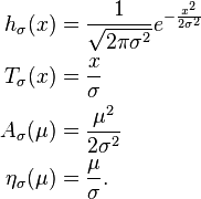
As a first example, consider a random variable distributed normally with unknown mean μ and known variance σ2. The probability density function is then
This is a single-parameter exponential family, as can be seen by setting
If σ = 1 this is in canonical form, as then η(μ) = μ.
Normal distribution: unknown mean and unknown variance
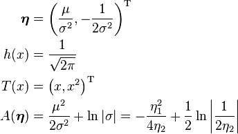
Next, consider the case of a normal distribution with unknown mean and unknown variance. The probability density function is then
This is an exponential family which can be written in canonical form by defining
Binomial distribution
As an example of a discrete exponential family, consider the binomial distribution with known number of trials n. The probability mass function for this distribution is
This can equivalently be written as
which shows that the binomial distribution is an exponential family, whose natural parameter is
This function of p is known as logit.
Table of distributions
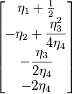
The following table shows how to rewrite a number of common distributions as exponential-family distributions with natural parameters. Refer to the flashcards[6] for main exponential families.
For a scalar variable and scalar parameter, the form is as follows:
For a scalar variable and vector parameter:
For a vector variable and vector parameter:
The above formulas choose the functional form of the exponential-family with a log-partition function  . The reason for this is so that the moments of the sufficient statistics can be calculated easily, simply by differentiating this function. Alternative forms involve either parameterizing this function in terms of the normal parameter
  instead of the natural parameter, and/or using a factor
  outside of the exponential. The relation between the latter and the former is:
To convert between the representations involving the two types of parameter, use the formulas below for writing one type of parameter in terms of the other.
| Distribution | Parameter(s) | Natural parameter(s) | Inverse parameter mapping | Base measure  | Sufficient statistic  | Log-partition  | Log-partition  |
|---|---|---|---|---|---|---|---|
| Bernoulli distribution | p | 
|

|
 |
 |
 |
 |
| binomial distribution with known number of trials n | p |  |
 |
 |
 |
 |
 |
| Poisson distribution | λ |  |
 |
 |
 |
 |
 |
| negative binomial distribution with known number of failures r | p |  |
 |
 |
 |
 |
 |
| exponential distribution | λ |  |
 |
 |
 |
 |
 |
| Pareto distribution with known minimum value xm | α |  |
 |
 |
 |
 |
 |
| Weibull distribution with known shape k | λ |  |
 |
 |
 |
 |
 |
| Laplace distribution with known mean μ | b |  |
 |
 |
 |
 |
 |
| chi-squared distribution | ν |  |
 |
 |
 |
 |
 |
| normal distribution known variance | μ |  |
 |
 |
 |
 |
 |
| normal distribution | μ,σ2 | ![\begin{bmatrix} \dfrac{\mu}{\sigma^2} \\[10pt] -\dfrac{1}{2\sigma^2} \end{bmatrix}](../I/m/28b2b8e29f38182accbf759b7d6e1451.png) |
![\begin{bmatrix} -\dfrac{\eta_1}{2\eta_2} \\[15pt] -\dfrac{1}{2\eta_2} \end{bmatrix}](../I/m/6ca21e6a838437db230f4c89622d47e8.png) |
 |
 |
 |
 |
| lognormal distribution | μ,σ2 | ![\begin{bmatrix} \dfrac{\mu}{\sigma^2} \\[10pt] -\dfrac{1}{2\sigma^2} \end{bmatrix}](../I/m/28b2b8e29f38182accbf759b7d6e1451.png) |
![\begin{bmatrix} -\dfrac{\eta_1}{2\eta_2} \\[15pt] -\dfrac{1}{2\eta_2} \end{bmatrix}](../I/m/6ca21e6a838437db230f4c89622d47e8.png) |
 |
 |
 |
 |
| inverse Gaussian distribution | μ,λ | ![\begin{bmatrix} -\dfrac{\lambda}{2\mu^2} \\[15pt] -\dfrac{\lambda}{2} \end{bmatrix}](../I/m/a4e807546a1af5b43d38093d87863e90.png) |
![\begin{bmatrix} \sqrt{\dfrac{\eta_2}{\eta_1}} \\[15pt] -2\eta_2 \end{bmatrix}](../I/m/c6fe53944315a3b002a3f8b04bac6e53.png) |
 |
![\begin{bmatrix} x \\[5pt] \dfrac{1}{x} \end{bmatrix}](../I/m/77dd1db32564b91552679aff1475f133.png) |
 |
 |
| gamma distribution | α,β |  |
 |
 |
 |
 |
 |
| k, θ | ![\begin{bmatrix} k-1 \\[5pt] -\dfrac{1}{\theta} \end{bmatrix}](../I/m/0e65cc0a4617bf57b36b907f564fd6db.png) |
![\begin{bmatrix} \eta_1+1 \\[5pt] -\dfrac{1}{\eta_2} \end{bmatrix}](../I/m/ce1fa51bc7edf726ea21185f3cbfa3ba.png) |
 | ||||
| inverse gamma distribution | α,β |  |
 |
 |
 |
 |
 |
| scaled inverse chi-squared distribution | ν,σ2 | ![\begin{bmatrix} -\dfrac{\nu}{2}-1 \\[10pt] -\dfrac{\nu\sigma^2}{2} \end{bmatrix}](../I/m/ab44bdf79b4c1171dad9cf9c430a0c69.png) |
![\begin{bmatrix} -2(\eta_1+1) \\[10pt] \dfrac{\eta_2}{\eta_1+1} \end{bmatrix}](../I/m/ae76a1712b11052510ae4ada719fba4b.png) |
 |
 |
 |
 |
| beta distribution | α,β |  |
 |
 |
 |
 |
 |
| multivariate normal distribution | μ,Σ | ![\begin{bmatrix} \boldsymbol\Sigma^{-1}\boldsymbol\mu \\[5pt] -\frac12\boldsymbol\Sigma^{-1} \end{bmatrix}](../I/m/e549f4542b9b021e8bc18bb7cacdd92f.png) |
![\begin{bmatrix} -\frac12\boldsymbol\eta_2^{-1}\boldsymbol\eta_1 \\[5pt] -\frac12\boldsymbol\eta_2^{-1} \end{bmatrix}](../I/m/6f65be0fdb67ae38c3bc8ca02b056f2c.png) |
 |
![\begin{bmatrix} \mathbf{x} \\[5pt] \mathbf{x}\mathbf{x}^\mathrm{T} \end{bmatrix}](../I/m/acbeb9e563e4102f8c6a0faaf43be985.png) |
 |
 |
| categorical distribution (variant 1) | p1,...,pk where  |
 |
 where  |
 |
![\begin{bmatrix} [x=1] \\ \vdots \\ {[x=k]} \end{bmatrix}](../I/m/edddbfd465936a22977039b73d6a96c6.png)
|
 |
 |
| categorical distribution (variant 2) | p1,...,pk where  |
 |

where |
 |
![\begin{bmatrix} [x=1] \\ \vdots \\ {[x=k]} \end{bmatrix}](../I/m/edddbfd465936a22977039b73d6a96c6.png)
|
 |
 |
| categorical distribution (variant 3) | p1,...,pk where  |
![\begin{bmatrix} \ln \dfrac{p_1}{p_k} \\[10pt] \vdots \\[5pt] \ln \dfrac{p_{k-1}}{p_k} \\[15pt] 0 \end{bmatrix} =](../I/m/b123fd9bc93cdbba08f4b8c4f2db9a17.png) ![\begin{bmatrix} \ln \dfrac{p_1}{1-\sum_{i=1}^{k-1}p_i} \\[10pt] \vdots \\[5pt] \ln \dfrac{p_{k-1}}{1-\sum_{i=1}^{k-1}p_i} \\[15pt] 0 \end{bmatrix}](../I/m/9bf22e441fa11cd651b466c89aefa82c.png)
|
![\begin{bmatrix} \dfrac{e^{\eta_1}}{\sum_{i=1}^{k}e^{\eta_i}} \\[10pt] \vdots \\[5pt] \dfrac{e^{\eta_k}}{\sum_{i=1}^{k}e^{\eta_i}} \end{bmatrix} =](../I/m/8139ce090eb15313b43ff88b44fbc685.png)
|
 |
![\begin{bmatrix} [x=1] \\ \vdots \\ {[x=k]} \end{bmatrix}](../I/m/edddbfd465936a22977039b73d6a96c6.png)
|
 |
 |
| multinomial distribution (variant 1) with known number of trials n | p1,...,pk where  |
 |
 where  |
 |
 |
 |
 |
| multinomial distribution (variant 2) with known number of trials n | p1,...,pk where  |
 |

where |
 |
 |
 |
 |
| multinomial distribution (variant 3) with known number of trials n |
p1,...,pk where  |
![\begin{bmatrix} \ln \dfrac{p_1}{p_k} \\[10pt] \vdots \\[5pt] \ln \dfrac{p_{k-1}}{p_k} \\[15pt] 0 \end{bmatrix} =](../I/m/b123fd9bc93cdbba08f4b8c4f2db9a17.png) ![\begin{bmatrix} \ln \dfrac{p_1}{1-\sum_{i=1}^{k-1}p_i} \\[10pt] \vdots \\[5pt] \ln \dfrac{p_{k-1}}{1-\sum_{i=1}^{k-1}p_i} \\[15pt] 0 \end{bmatrix}](../I/m/9bf22e441fa11cd651b466c89aefa82c.png) |
![\begin{bmatrix} \dfrac{e^{\eta_1}}{\sum_{i=1}^{k}e^{\eta_i}} \\[10pt] \vdots \\[5pt] \dfrac{e^{\eta_k}}{\sum_{i=1}^{k}e^{\eta_i}} \end{bmatrix} =](../I/m/8139ce090eb15313b43ff88b44fbc685.png)
|
 |
 |
 |
 |
| Dirichlet distribution | α1,...,αk |  |
 |
 |
 |
 |
 |
| Wishart distribution | V,n | ![\begin{bmatrix} -\frac12\mathbf{V}^{-1} \\[5pt] \dfrac{n-p-1}{2} \end{bmatrix}](../I/m/c33917bd64fd3b22d85189378b8365a5.png) |
![\begin{bmatrix} -\frac12{\boldsymbol\eta_1}^{-1} \\[5pt] 2\eta_2+p+1 \end{bmatrix}](../I/m/d78fc1c30ebecebf81cc7f6cea41b38a.png) |
 |
 |

|
 |
NOTE: Uses the fact that  i.e. the trace of a matrix product is much like a dot product. The matrix parameters are assumed to be vectorized (laid out in a vector) when inserted into the exponential form. Also, V and X are symmetric, so e.g. i.e. the trace of a matrix product is much like a dot product. The matrix parameters are assumed to be vectorized (laid out in a vector) when inserted into the exponential form. Also, V and X are symmetric, so e.g.  | |||||||
| inverse Wishart distribution | Ψ,m | ![\begin{bmatrix} -\frac12\boldsymbol\Psi \\[5pt] -\dfrac{m+p+1}{2} \end{bmatrix}](../I/m/b4ec448b0af18cfb79bac549c3ecfac8.png) |
![\begin{bmatrix} -2\boldsymbol\eta_1 \\[5pt] -(2\eta_2+p+1) \end{bmatrix}](../I/m/2d14851f6f178d756697be2e4e339347.png) |
 |
 |
 |
 |
| normal-gamma distribution | α,β,μ,λ | 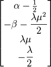 |
 |
 |
 |
 |
 |
The three variants of the categorical distribution and multinomial distribution are due to the fact that the parameters  are constrained, such that
Thus, there are only k−1 independent parameters.
- Variant 1 uses k natural parameters with a simple relation between the standard and natural parameters; however, only k−1 of the natural parameters are independent, and the set of k natural parameters is nonidentifiable. The constraint on the usual parameters translates to a similar constraint on the natural parameters.
- Variant 2 demonstrates the fact that the entire set of natural parameters is nonidentifiable: Adding any constant value to the natural parameters has no effect on the resulting distribution. However, by using the constraint on the natural parameters, the formula for the normal parameters in terms of the natural parameters can be written in a way that is independent on the constant that is added.
- Variant 3 shows how to make the parameters identifiable in a convenient way by setting
 This effectively "pivots" around pk and causes the last natural parameter to have the constant value of 0. All the remaining formulas are written in a way that does not access pk, so that effectively the model has only k−1 parameters, both of the usual and natural kind.
Note also that variants 1 and 2 are not actually standard exponential families at all. Rather they are curved exponential families, i.e. there are k−1 independent parameters embedded in a k-dimensional parameter space. Many of the standard results for exponential families do not apply to curved exponential families. An example is the log-partition function A(x), which has the value of 0 in the curved cases. In standard exponential families, the derivatives of this function correspond to the moments (more technically, the cumulants) of the sufficient statistics, e.g. the mean and variance. However, a value of 0 suggests that the mean and variance of all the sufficient statistics are uniformly 0, whereas in fact the mean of the ith sufficient statistic should be pi. (This does emerge correctly when using the form of A(x) in variant 3.)
Moments and cumulants of the sufficient statistic
Normalization of the distribution
We start with the normalization of the probability distribution. In general, an arbitrary function f(x) that serves as the kernel of a probability distribution (the part encoding all dependence on x) can be made into a proper distribution by normalizing: i.e.
where
The factor Z is sometimes termed the normalizer or partition function, based on an analogy to statistical physics.
In the case of an exponential family where
the kernel is
and the partition function is
Since the distribution must be normalized, we have
In other words,
or equivalently
This justifies calling A the log-normalizer or log-partition function.
Moment generating function of the sufficient statistic
Now, the moment generating function of T(x) is
proving the earlier statement that
is the cumulant generating function for T.
An important subclass of the exponential family the natural exponential family has a similar form for the moment generating function for the distribution of x.
Differential identities for cumulants
In particular, using the properties of the cumulant generating function,
and
The first two raw moments and all mixed second moments can be recovered from these two identities. Higher order moments and cumulants are obtained by higher derivatives. This technique is often useful when T is a complicated function of the data, whose moments are difficult to calculate by integration.
Another way to see this that does not rely on the theory of cumulants is to begin from the fact that the distribution of an exponential family must be normalized, and differentiate. We illustrate using the simple case of a one-dimensional parameter, but an analogous derivation holds more generally.
In the one-dimensional case, we have
This must be normalized, so
Take the derivative of both sides with respect to η:
Therefore,
Example 1
As an introductory example, consider the gamma distribution, whose distribution is defined by
Referring to the above table, we can see that the natural parameter is given by
the reverse substitutions are
the sufficient statistics are  and the log-partition function is
We can find the mean of the sufficient statistics as follows. First, for η1:
Where  is the digamma function (derivative of log gamma), and we used the reverse substitutions in the last step.
Now, for η2:
again making the reverse substitution in the last step.
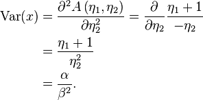
To compute the variance of x, we just differentiate again:
All of these calculations can be done using integration, making use of various properties of the gamma function, but this requires significantly more work.
Example 2
As another example consider a real valued random variable X with density
indexed by shape parameter  (this is called the skew-logistic distribution). The density can be rewritten as
Notice this is an exponential family with natural parameter
sufficient statistic
and log-partition function
So using the first identity,
and using the second identity
This example illustrates a case where using this method is very simple, but the direct calculation would be nearly impossible.
Example 3
The final example is one where integration would be extremely difficult. This is the case of the Wishart distribution, which is defined over matrices. Even taking derivatives is a bit tricky, as it involves matrix calculus, but the respective identities are listed in that article.
From the above table, we can see that the natural parameter is given by
the reverse substitutions are
and the sufficient statistics are 
The log-partition function is written in various forms in the table, to facilitate differentiation and back-substitution. We use the following forms:
- Expectation of X (associated with η1)
To differentiate with respect to η1, we need the following matrix calculus identity:
Then:
The last line uses the fact that V is symmetric, and therefore it is the same when transposed.
- Expectation of ln |X| (associated with η2)
Now, for η2, we first need to expand the part of the log-partition function that involves the multivariate gamma function:
We also need the digamma function:
Then:
This latter formula is listed in the Wishart distribution article. Both of these expectations are needed when deriving the variational Bayes update equations in a Bayes network involving a Wishart distribution (which is the conjugate prior of the multivariate normal distribution).
Computing these formulas using integration would be much more difficult. The first one, for example, would require matrix integration.
Maximum entropy derivation
The exponential family arises naturally as the answer to the following question: what is the maximum-entropy distribution consistent with given constraints on expected values?
The information entropy of a probability distribution dF(x) can only be computed with respect to some other probability distribution (or, more generally, a positive measure), and both measures must be mutually absolutely continuous. Accordingly, we need to pick a reference measure dH(x) with the same support as dF(x).
The entropy of dF(x) relative to dH(x) is
or
where dF/dH and dH/dF are Radon–Nikodym derivatives. Note that the ordinary definition of entropy for a discrete distribution supported on a set I, namely
assumes, though this is seldom pointed out, that dH is chosen to be the counting measure on I.
Consider now a collection of observable quantities (random variables) Ti. The probability distribution dF whose entropy with respect to dH is greatest, subject to the conditions that the expected value of Ti be equal to ti, is a member of the exponential family with dH as reference measure and (T1, ..., Tn) as sufficient statistic.
The derivation is a simple variational calculation using Lagrange multipliers. Normalization is imposed by letting T0 = 1 be one of the constraints. The natural parameters of the distribution are the Lagrange multipliers, and the normalization factor is the Lagrange multiplier associated to T0.
For examples of such derivations, see Maximum entropy probability distribution.
Role in statistics
Classical estimation: sufficiency
According to the Pitman–Koopman–Darmois theorem, among families of probability distributions whose domain does not vary with the parameter being estimated, only in exponential families is there a sufficient statistic whose dimension remains bounded as sample size increases.
Less tersely, suppose Xk, (where k = 1, 2, 3, ... n) are independent, identically distributed random variables. Only if their distribution is one of the exponential family of distributions is there a sufficient statistic T(X1, ..., Xn) whose number of scalar components does not increase as the sample size n increases; the statistic T may be a vector or a single scalar number, but whatever it is, its size will neither grow nor shrink when more data are obtained.
Bayesian estimation: conjugate distributions
Exponential families are also important in Bayesian statistics. In Bayesian statistics a prior distribution is multiplied by a likelihood function and then normalised to produce a posterior distribution. In the case of a likelihood which belongs to the exponential family there exists a conjugate prior, which is often also in the exponential family. A conjugate prior π for the parameter  of an exponential family
is given by
or equivalently
where s is the dimension of  and
and  and
and  are hyperparameters (parameters controlling parameters). ν corresponds to the effective number of observations that the prior distribution contributes, and
  corresponds to the total amount that these pseudo-observations contribute to the sufficient statistic over all observations and pseudo-observations.
  is a normalization constant that is automatically determined by the remaining functions and serves to ensure that the given function is a probability density function (i.e. it is normalized).
  and equivalently
  are the same functions as in the definition of the distribution over which π is the conjugate prior.
A conjugate prior is one which, when combined with the likelihood and normalised, produces a posterior distribution which is of the same type as the prior. For example, if one is estimating the success probability of a binomial distribution, then if one chooses to use a beta distribution as one's prior, the posterior is another beta distribution. This makes the computation of the posterior particularly simple. Similarly, if one is estimating the parameter of a Poisson distribution the use of a gamma prior will lead to another gamma posterior. Conjugate priors are often very flexible and can be very convenient. However, if one's belief about the likely value of the theta parameter of a binomial is represented by (say) a bimodal (two-humped) prior distribution, then this cannot be represented by a beta distribution. It can however be represented by using a mixture density as the prior, here a combination of two beta distributions; this is a form of hyperprior.
An arbitrary likelihood will not belong to the exponential family, and thus in general no conjugate prior exists. The posterior will then have to be computed by numerical methods.
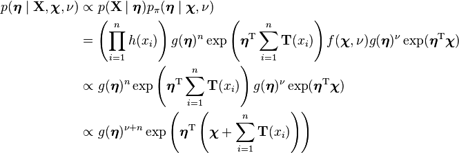
To show that the above prior distribution is a conjugate prior, we can derive the posterior.
First, assume that the probability of a single observation follows an exponential family, parameterized using its natural parameter:
Then, for data  , the likelihood is computed as follows:
Then, for the above conjugate prior:
We can then compute the posterior as follows:
The last line is the kernel of the prior distribution, i.e.
This shows that the posterior has the same form as the prior.
Note in particular that the data X enters into this equation only in the expression
which is termed the sufficient statistic of the data. That is, the value of the sufficient statistic is sufficient to completely determine the posterior distribution. The actual data points themselves are not needed, and all sets of data points with the same sufficient statistic will have the same distribution. This is important because the dimension of the sufficient statistic does not grow with the data size — it has only as many components as the components of  (equivalently, the number of parameters of the distribution of a single data point).
The update equations are as follows:
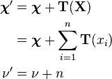
This shows that the update equations can be written simply in terms of the number of data points and the sufficient statistic of the data. This can be seen clearly in the various examples of update equations shown in the conjugate prior page. Note also that because of the way that the sufficient statistic is computed, it necessarily involves sums of components of the data (in some cases disguised as products or other forms — a product can be written in terms of a sum of logarithms). The cases where the update equations for particular distributions don't exactly match the above forms are cases where the conjugate prior has been expressed using a different parameterization than the one that produces a conjugate prior of the above form — often specifically because the above form is defined over the natural parameter  while conjugate priors are usually defined over the actual parameter
Hypothesis testing: uniformly most powerful tests
The one-parameter exponential family has a monotone non-decreasing likelihood ratio in the sufficient statistic T(x), provided that η(θ) is non-decreasing. As a consequence, there exists a uniformly most powerful test for testing the hypothesis H0: θ ≥ θ0 vs. H1: θ < θ0.
Generalized linear models
The exponential family forms the basis for the distribution function used in generalized linear models, a class of model that encompass many of the commonly used regression models in statistics.
See also
References
- ↑ Andersen, Erling (September 1970). "Sufficiency and Exponential Families for Discrete Sample Spaces". Journal of the American Statistical Association (Journal of the American Statistical Association, Vol. 65, No. 331) 65 (331): 1248–1255. doi:10.2307/2284291. JSTOR 2284291. MR 268992.
- ↑ Pitman, E.; Wishart, J. (1936). "Sufficient statistics and intrinsic accuracy". Mathematical Proceedings of the Cambridge Philosophical Society 32 (4): 567–579. doi:10.1017/S0305004100019307.
- ↑ Darmois, G. (1935). "Sur les lois de probabilites a estimation exhaustive". C.R. Acad. Sci. Paris (in French) 200: 1265–1266.
- ↑ Koopman, B (1936). "On distribution admitting a sufficient statistic". Transactions of the American Mathematical Society (Transactions of the American Mathematical Society, Vol. 39, No. 3) 39 (3): 399–409. doi:10.2307/1989758. JSTOR 1989758. MR 1501854.
- ↑ Kupperman, M. (1958) "Probabilities of Hypotheses and Information-Statistics in Sampling from Exponential-Class Populations", Annals of Mathematical Statistics, 9 (2), 571–575 JSTOR 2237349
- ↑ Nielsen, Frank; Garcia, Vincent (2009). "Statistical exponential families: A digest with flash cards". arxiv (0911.4863).
Further reading
- Lehmann, E. L.; Casella, G. (1998). Theory of Point Estimation. pp. 2nd ed., sec. 1.5.
- Keener, Robert W. (2006). Statistical Theory: Notes for a Course in Theoretical Statistics. Springer. pp. 27–28, 32–33.
- Fahrmeier, Ludwig; Tutz, G. (1994). Multivariate statistical modelling based on generalized linear models. Springer. pp. 18–22, 345–349.
External links
- A primer on the exponential family of distributions
- Exponential family of distributions on the Earliest known uses of some of the words of mathematics
- jMEF: A Java library for exponential families


![f(x), g(\theta), c^{f(x)}, c^{g(\theta)}, {[f(x)]}^c, {[g(\theta)]}^c, {[f(x)]}^{g(\theta)}, {[g(\theta)]}^{f(x)}, {[f(x)]}^{h(x)g(\theta)}, \text{ or } {[g(\theta)]}^{h(x)j(\theta)},](../I/m/d545b3d0e4786a376c041a729cb5208c.png)
![{[f(x) g(\theta)]}^{h(x)j(\theta)}, \qquad {[f(x)]}^{h(x)j(\theta)} [g(\theta)]^{h(x)j(\theta)},](../I/m/5df277d9480981a4703e2d3a827ca09e.png)
![{[f(x) g(\theta)]}^{h(x)j(\theta)} = {[f(x)]}^{h(x)j(\theta)} [g(\theta)]^{h(x)j(\theta)} = e^{[h(x) \ln f(x)] j(\theta) + h(x) [j(\theta) \ln g(\theta)]},](../I/m/e63b1b5477c64bed888625e1d138c9e9.png)
![{[f(x)]}^{g(\theta)}](../I/m/3700f25289321f2eeef7918bdfccfba7.png)
![{[f(x)]}^{g(\theta)} = e^{g(\theta) \ln f(x)}](../I/m/8da4ecdaaa09aad3a91f24cf51b215f6.png)
![{[f(x)]}^{h(x)g(\theta)} = e^{h(x)g(\theta)\ln f(x)} = e^{[h(x) \ln f(x)] g(\theta)}](../I/m/a8eddd3f4db5521a2b055f33e97a9c13.png)





![[x=i]](../I/m/2bd4b55c9539155fb4b0da36be8424a1.png) is the
is the  , 0 otherwise).
![\begin{bmatrix} \dfrac{e^{\eta_1}}{\sum_{i=1}^{k}e^{\eta_i}} \\[10pt] \vdots \\[5pt] \dfrac{e^{\eta_k}}{\sum_{i=1}^{k}e^{\eta_i}} \end{bmatrix}](../I/m/7b0bcd74f36842e032bbc3acc24d55fe.png)

![\begin{bmatrix} \dfrac{e^{\eta_1}}{1+\sum_{i=1}^{k-1}e^{\eta_i}} \\[10pt] \vdots \\[5pt] \dfrac{e^{\eta_{k-1}}}{1+\sum_{i=1}^{k-1}e^{\eta_i}} \\[15pt] \dfrac{1}{1+\sum_{i=1}^{k-1}e^{\eta_i}} \end{bmatrix}](../I/m/3f93a9d7e3d46b3769bca7d6181bb0d7.png)


![M_T(u) \equiv E[e^{u^{\rm T} T(x)}\mid\eta] = \int_x h(x) e^{(\eta+u)^{\rm T} T(x)-A(\eta)} dx = e^{A(\eta + u)-A(\eta)}](../I/m/b2a92e75430824f441f0e71418d35a1b.png)


![\begin{align}
0 &= g(\eta) \frac{d}{d\eta} \int_x h(x) e^{\eta T(x)} dx + g'(\eta)\int_x h(x) e^{\eta T(x)} dx \\
&= g(\eta) \int_x h(x) \left(\frac{d}{d\eta} e^{\eta T(x)}\right) dx + g'(\eta)\int_x h(x) e^{\eta T(x)} dx \\
&= g(\eta) \int_x h(x) e^{\eta T(x)} T(x) dx + g'(\eta)\int_x h(x) e^{\eta T(x)} dx \\
&= \int_x T(x) g(\eta) h(x) e^{\eta T(x)} dx + \frac{g'(\eta)}{g(\eta)}\int_x g(\eta) h(x) e^{\eta T(x)} dx \\
&= \int_x T(x) p(x) dx + \frac{g'(\eta)}{g(\eta)}\int_x p(x) dx \\
&= \mathbb{E}[T(x)] + \frac{g'(\eta)}{g(\eta)} \\
&= \mathbb{E}[T(x)] + \frac{d}{d\eta} \ln g(\eta)
\end{align}](../I/m/11f6197c841abca4770fe7ef440ec962.png)
![\mathbb{E}[T(x)] = - \frac{d}{d\eta} \ln g(\eta) = \frac{d}{d\eta} A(\eta).](../I/m/bdf61e258af95019506c2d9377788e45.png)


![\begin{align}
\mathbb{E}[\ln x] &= \frac{ \partial A(\eta_1,\eta_2) }{ \partial \eta_1 } = \frac{ \partial }{ \partial \eta_1 } \left(\ln\Gamma(\eta_1+1) - (\eta_1+1) \ln(-\eta_2)\right) \\
&= \psi(\eta_1+1) - \ln(-\eta_2) \\
&= \psi(\alpha) - \ln \beta,
\end{align}](../I/m/357c66f07e49e18364d27fda1e1b68e4.png)
![\begin{align}
\mathbb{E}[x] &= \frac{ \partial A(\eta_1,\eta_2) }{ \partial \eta_2 } = \frac{ \partial }{ \partial \eta_2 } \left(\ln \Gamma(\eta_1+1)-(\eta_1+1)\ln(-\eta_2)\right) \\
&= -(\eta_1+1)\frac{1}{-\eta_2}(-1) = \frac{\eta_1+1}{-\eta_2} \\
&= \frac{\alpha}{\beta},
\end{align}](../I/m/adc9dbb5b7b1866e56287dfaf48feb1e.png)


![E(\log(1 + e^{-X})) = E(T) = \frac{ \partial A(\eta) }{ \partial \eta } = \frac{ \partial }{ \partial \eta } [-\log(-\eta)] = \frac{1}{-\eta} = \frac{1}{\theta},](../I/m/27832487e4e82360bbe55c71ddbe01da.png)
![\mathrm{var}(\log\left(1 + e^{-X} \right)) = \frac{ \partial^2 A(\eta) }{ \partial \eta^2 } = \frac{ \partial }{ \partial \eta } \left[\frac{1}{-\eta}\right] = \frac{1}{(-\eta)^2} = \frac{1}{\theta^2}.](../I/m/42823e10212a5ee02790e19866c1374e.png)


![\begin{align}
\mathbb{E}[\mathbf{X}] &= \frac{ \partial A\left(\boldsymbol\eta_1,\cdots \right) }{ \partial \boldsymbol\eta_1 } \\
&= \frac{ \partial }{ \partial \boldsymbol\eta_1 } \left[-\frac{n}{2}\ln|-\boldsymbol\eta_1| + \ln\Gamma_p\left(\frac{n}{2}\right) \right] \\
&= -\frac{n}{2}(\boldsymbol\eta_1^{-1})^{\rm T} \\
&= \frac{n}{2}(-\boldsymbol\eta_1^{-1})^{\rm T} \\
&= n(\mathbf{V})^{\rm T} \\
&= n\mathbf{V}
\end{align}](../I/m/a380e888161a6105fa0f59df29cca1d2.png)
![\ln \Gamma_p(a)= \ln \left(\pi^{\frac{p(p-1)}{4}}\prod_{j=1}^p \Gamma\left(a+\frac{1-j}{2}\right)\right) = \frac{p(p-1)}{4} \ln \pi + \sum_{j=1}^p \ln \Gamma\left[ a+\frac{1-j}{2}\right]](../I/m/d0c55a6a8268e9b199a6773d672a28cc.png)

![\begin{align}
\mathbb{E}[\ln |\mathbf{X}|] &= \frac{\partial A\left (\cdots,\eta_2 \right)}{\partial \eta_2} \\
&= \frac{\partial}{\partial \eta_2} \left[-\left(\eta_2+\frac{p+1}{2}\right)(p\ln 2 + \ln|\mathbf{V}|) + \ln\Gamma_p\left(\eta_2+\frac{p+1}{2}\right) \right] \\
&= \frac{\partial}{\partial \eta_2} \left[ \left(\eta_2+\frac{p+1}{2}\right)(p\ln 2 + \ln|\mathbf{V}|) + \frac{p(p-1)}{4} \ln \pi + \sum_{j=1}^p \ln \Gamma\left(\eta_2+\frac{p+1}{2}+\frac{1-j}{2}\right) \right] \\
&= p\ln 2 + \ln|\mathbf{V}| + \sum_{j=1}^p \psi\left(\eta_2+\frac{p+1}{2}+\frac{1-j}{2}\right) \\
&= p\ln 2 + \ln|\mathbf{V}| + \sum_{j=1}^p \psi\left(\frac{n-p-1}{2}+\frac{p+1}{2}+\frac{1-j}{2}\right) \\
&= p\ln 2 + \ln|\mathbf{V}| + \sum_{j=1}^p \psi\left(\frac{n+1-j}{2}\right)
\end{align}](../I/m/6b979fea27ba4b3240481250fa5d397c.png)
![S[dF\mid dH]=-\int \frac{dF}{dH}\ln\frac{dF}{dH}\,dH](../I/m/536df62a7c22ed49c4b0c29498d1386e.png)
![S[dF\mid dH]=\int\ln\frac{dH}{dF}\,dF](../I/m/a418e60c20de043c73fd13c0fe202af3.png)


