Laplace's method
See also: Additive smoothing (Laplace smoothing) a method of smoothing of a statistical estimator
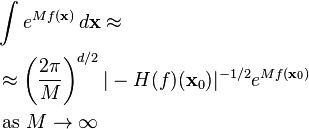
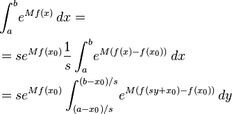
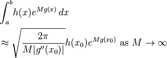
In mathematics, Laplace's method, named after Pierre-Simon Laplace, is a technique used to approximate integrals of the form
where ƒ(x) is some twice-differentiable function, M is a large number, and the integral endpoints a and b could possibly be infinite. This technique was originally presented in Laplace (1774, pp. 366–367).
The idea of Laplace's method

Assume that the function ƒ(x) has a unique global maximum at x0. Then, the value ƒ(x0) will be larger than other values ƒ(x). If we multiply this function by a large number M, the ratio between Mƒ(x0) and Mƒ(x) will stay the same (since Mƒ(x0)/Mƒ(x) = ƒ(x0)/ƒ(x)), but it will grow exponentially in the function (see figure)
Thus, significant contributions to the integral of this function will come only from points x in a neighborhood of x0, which can then be estimated.
General theory of Laplace's method
To state and motivate the method, we need several assumptions. We will assume that x0 is not an endpoint of the interval of integration, that the values ƒ(x) cannot be very close to ƒ(x0) unless x is close to x0, and that the second derivative  .
.
We can expand ƒ(x) around x0 by Taylor's theorem,
where 
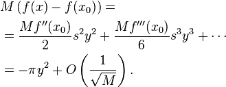
Since ƒ has a global maximum at x0, and since x0 is not an endpoint, it is a stationary point, so the derivative of ƒ vanishes at x0. Therefore, the function ƒ(x) may be approximated to quadratic order
for x close to x0 (recall that the second derivative is negative at the global maximum ƒ(x0)). The assumptions made ensure the accuracy of the approximation
(see the picture on the right). This latter integral is a Gaussian integral if the limits of integration go from −∞ to +∞ (which can be assumed because the exponential decays very fast away from x0), and thus it can be calculated. We find
A generalization of this method and extension to arbitrary precision is provided by Fog (2008).
Formal statement and proof:
Assume that  is a twice differentiable function on
 ![[a,b]](../I/m/2c3d331bc98b44e71cb2aae9edadca7e.png) with
with ![x_0 \in [a,b]](../I/m/0256d46865eafa8df913009bb4f1d987.png) the unique point such that
the unique point such that ![f(x_0) = \max_{[a,b]} f(x)](../I/m/8f088a9931ae52355734e1cf773fc915.png) . Assume additionally that
. Assume additionally that  .
.
Then,
Lower bound:
Let  . Then by the continuity of
  there exists
  such that if
  then
then  . By Taylor's Theorem, for any
  ,
,  .
.
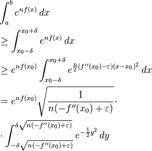
Then we have the following lower bound:
where the last equality was obtained by a change of variables  . Remember that
  so that is why we can take the square root of its negation.
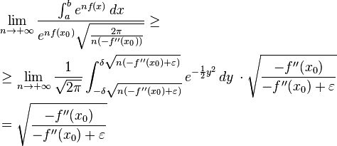
If we divide both sides of the above inequality by  and take the limit we get:
since this is true for arbitrary  we get the lower bound:
Note that this proof works also when  or
or  (or both).
Upper bound:
The proof of the upper bound is similar to the proof of the lower bound but there are a few inconveniences. Again we start by picking an  but in order for the proof to work we need
  small enough so that
  . Then, as above, by continuity of
  and Taylor's Theorem we can find
  so that if
  , then
  . Lastly, by our assumptions (assuming
  are finite) there exists an
  such that if
  , then
  .
.
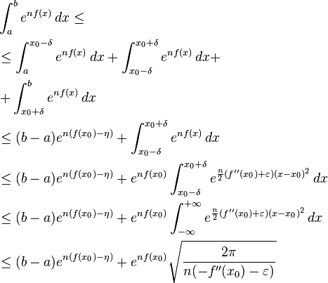
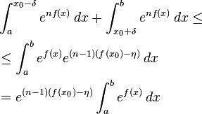
Then we can calculate the following upper bound:
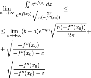
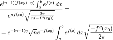
If we divide both sides of the above inequality by  and take the limit we get:
Since  is arbitrary we get the upper bound:
And combining this with the lower bound gives the result.
Note that the above proof obviously fails when  or
or  (or both). To deal with these cases, we need some extra assumptions. A sufficient (not necessary) assumption is that for
  , the integral
  is finite, and that the number
  as above exists (note that this must be an assumption in the case when the interval
 ![[a,b]](../I/m/2c3d331bc98b44e71cb2aae9edadca7e.png) is infinite). The proof proceeds otherwise as above, but the integrals
is infinite). The proof proceeds otherwise as above, but the integrals
must be approximated by
instead of  as above, so that when we divide by
  , we get for this term
whose limit as  is
is  . The rest of the proof (the analysis of the interesting term) proceeds as above.
The given condition in the infinite interval case is, as said above, sufficient but not necessary. However, the condition is fulfilled in many, if not in most, applications: the condition simply says that the integral we are studying must be well-defined (not infinite) and that the maximum of the function at  must be a "true" maximum (the number
  must exist). There is no need to demand that the integral is finite for
  but it is enough to demand that the integral is finite for some
  .
.
This method relies on 4 basic concepts such as
- 1. Relative error
First of all, we need to have an understanding about the so-called “approximation” in this method is related to the relative error instead of the absolute error. Therefore, if we set

, this integration can be written as
, where  is a small number when
  is a large number obviously and the relative error will be
Now, let us separate this integration into two parts: ![y\in[-D_y,D_y]](../I/m/04a735a31d4646e1411414ba21f6f8eb.png) region and the rest part.
region and the rest part.
- 2. function
 will tend to
  around the stationary point when
  is large enough
Let’s look at the Taylor expansion of  around x0 and translate x to y because we do the comparison in y-space, we will get
Note that  because
  is a stationary point.
From this equation you will find that the terms higher than second derivative in this Taylor expansion is suppressed as the order of
  so that
  will get closer to the Gaussian function as shown in figure. Besides,

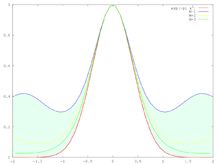
![e^{M[f(sy+x_0)-f(x_0)]}](../I/m/1e093abfe1c59f9be4169c84a470c779.png) with
with  equals 1, 2 and 3, and the red line is the curve of function
  .
.- 3. The bigger
 is, the smaller range of
  is related
Because we do the comparison in y-space,  is fixed in
 ![y\in[-D_y,D_y]](../I/m/04a735a31d4646e1411414ba21f6f8eb.png) which will cause
which will cause ![x\in[-sD_y,sD_y]](../I/m/0631b7db469f0c4770009527d5797593.png) ; however,
; however,  is inversely proportional to
  , the chosen region of
  will be smaller when
  is increased.
- 4. If the integration used by Laplace’s method is converged, the contribution of the region which is not around the stationary point
 of the integration of its relative error will tend to zero when
  is increased.
Relying on the 3rd concept, even if we choose a very large Dy , sDy will finally be a very small number when  is increased to a huge number. Then, how can we guarantee the integration of the rest part will tend to 0 when
  is large enough?
The basic idea is trying to find a function  which will
  and the integration of
  will tend to zero when
  is increased. Because the exponential function of
  will be always larger than zero as long as
  is a real number, and this exponential function is proportional to
  , the integration of
  will tend to zero. For simplicity, let me choose
  as a tangent through the point
  as shown in the figure:
.gif)
 is denoted by the two tangent lines passing through
  . When
  gets smaller, the cover region will be larger.
 If the interval of the integration of this method is finite, we will find that no matter  is continue in the rest region, it will be always smaller than
  shown above when
  is large enough. By the way, it will be proved later that the integration of
  will tend to zero when
  is large enough.
If the interval of the integration of this method is infinite,  and
and  might always cross to each other. If so, we cannot guarantee that the integration of
  will tend to zero finally. For example, in the case of
  ,
,  will be always diverged. Therefore, we need to require that
  can converge for the infinite interval case. If so, this integration will tend to zero when
  is large enough and we can choose this
  as the cross of
  and
and  .
.
You might ask that why not choose  as a convergent integration? Let me use an example to show you the reason. Suppose the rest part of
  is
is  , then
  and its integration will diverge; however, when
  ,the integration of
  converges. So, the integrations of some functions will diverge when
  is not a large number, but they will converge when
  is large enough.
Based on these four concepts, we can derive the relative error of this Laplace's method.
Other formulations
Laplace's approximation is sometimes written as
where  is positive.
Importantly, the accuracy of the approximation depends on the variable of integration, that is, on what stays in  and what goes into
  .[1]
.[1]
First of all, let me set the global maximum is located at  which can simplify the derivation and does not lost any important information; therefore, all the derivation inside this sub-section is under this assumption. Besides, what we want is the relative error
  as shown below
where  .
So, if we let
 ![A\equiv \frac{h(sy)}{h(0)}e^{M\left[g(sy)-g(0) \right]}](../I/m/e52bd7e089efd4b3c8053e8c25d198ff.png) and
and  , we can get
since  . Now, let us find its upper bound.
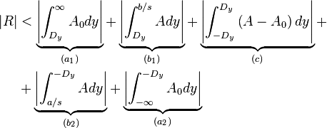
Owing to  , we can separate this integration into 5 parts with 3 different types (a), (b) and (c), respectively. Therefore,
where  and
and  are similar, let us just calculate
  , and
, and  and
and  are similar, too, I’ll just calculate
  .
.
For  , after the translation of
  , we can get
This means that as long as  is large enough, it will tend to zero.
For  , we can get
where
and  should have the same sign of
  during this region.
Let us choose
  as the tangent across the point at
  , i.e.
  which is shown in the figure
.gif)
 is the tangent lines across the point at
  .
.From this figure you can find that when  or
or  gets smaller, the region satisfies the above inequality will get larger. Therefore, if we want to find a suitable
  to cover the whole
  during the interval of
  ,
,  will have an upper limit. Besides, because the integration of
  is simple, let me use it to estimate the relative error contributed by this
  .
.
Based on Taylor expansion, we can get
and
and then substitute them back into the calculation of  ; however, you can find that the remainders of these two expansions are both inversely proportional to the square root of
  , let me drop them out to beautify the calculation. Keeping them is better, but it will make the formula uglier.
Therefore, it will tend to zero when  gets larger, but don't forget that the upper bound of
  should be considered during this calculation.
About the integration near  , we can also use Taylor's Theorem to calculate it. When
and you can find that it is inversely proportional to the square root of  . In fact,
  will have the same behave when
  is a constant.
Conclusively, the integration near the stationary point will get smaller when  gets larger, and the rest parts will tend to zero as long as
  is large enough; however, we need to remember that
  has an upper limit which is decided by whether the function
  is always larger than
  during this rest region. However, as long as we can find one
  satisfies this condition, the upper bound of
  can be chosen as directly proportional to
  since
since  is a tangent across the point of
  at
at  . So, the bigger
  is, the bigger
  can be.
In the multivariate case where  is a
is a  -dimensional vector and
  is a scalar function of
  , Laplace's approximation is usually written as:
where  is the Hessian matrix of
  evaluated at
  and where
  denotes matrix determinant. Analogously to the univariate case, the Hessian is required to be negative definite.[2]
By the way, although  denotes a
  -dimensional vector, the term
  denotes an Infinitesimal volume here, i.e.
  .
.
Laplace's method extension: Steepest descent
In extensions of Laplace's method, complex analysis, and in particular Cauchy's integral formula, is used to find a contour of steepest descent for an (asymptotically with large M) equivalent integral, expressed as a line integral. In particular, if no point x0 where the derivative of ƒ vanishes exists on the real line, it may be necessary to deform the integration contour to an optimal one, where the above analysis will be possible. Again the main idea is to reduce, at least asymptotically, the calculation of the given integral to that of a simpler integral that can be explicitly evaluated. See the book of Erdelyi (1956) for a simple discussion (where the method is termed steepest descents).
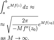
The appropriate formulation for the complex z-plane is
for a path passing through the saddle point at z0. Note the explicit appearance of a minus sign to indicate the direction of the second derivative: one must not take the modulus. Also note that if the integrand is meromorphic, one may have to add residues corresponding to poles traversed while deforming the contour (see for example section 3 of Okounkov's paper Symmetric functions and random partitions).
Further generalizations
An extension of the steepest descent method is the so-called nonlinear stationary phase/steepest descent method. Here, instead of integrals, one needs to evaluate asymptotically solutions of Riemann–Hilbert factorization problems.
Given a contour C in the complex sphere, a function ƒ defined on that contour and a special point, say infinity, one seeks a function M holomorphic away from the contour C, with prescribed jump across C, and with a given normalization at infinity. If ƒ and hence M are matrices rather than scalars this is a problem that in general does not admit an explicit solution.
An asymptotic evaluation is then possible along the lines of the linear stationary phase/steepest descent method. The idea is to reduce asymptotically the solution of the given Riemann–Hilbert problem to that of a simpler, explicitly solvable, Riemann–Hilbert problem. Cauchy's theorem is used to justify deformations of the jump contour.
The nonlinear stationary phase was introduced by Deift and Zhou in 1993, based on earlier work of Its. A (properly speaking) nonlinear steepest descent method was introduced by Kamvissis, K. McLaughlin and P. Miller in 2003, based on previous work of Lax, Levermore, Deift, Venakides and Zhou.
The nonlinear stationary phase/steepest descent method has applications to the theory of soliton equations and integrable models, random matrices and combinatorics.
Complex integrals
For complex integrals in the form:
with t >> 1, we make the substitution t = iu and the change of variable s = c + ix to get the bilateral Laplace transform:
We then split g(c+ix) in its real and complex part, after which we recover u = t / i. This is useful for inverse Laplace transforms, the Perron formula and complex integration.
Example 1: Stirling's approximation
Laplace's method can be used to derive Stirling's approximation
for a large integer N.
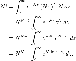
From the definition of the Gamma function, we have
Now we change variables, letting
so that
Plug these values back in to obtain
This integral has the form necessary for Laplace's method with
which is twice-differentiable:
The maximum of ƒ(z) lies at z0 = 1, and the second derivative of ƒ(z) has the value −1 at this point. Therefore, we obtain
Example 2: parameter estimation and probabilistic inference
Azevedo-Filho & Shachter 1994 reviews Laplace's method results (univariate and multivariate) and presents a detailed example showing the method used in parameter estimation and probabilistic inference under a Bayesian perspective. Laplace's method is applied to a meta-analysis problem from the medical domain, involving experimental data, and compared to other techniques.
See also
Notes
- ↑ Butler, Ronald W (2007). Saddlepoint approximations and applications. Cambridge University Press. ISBN 978-0-521-87250-8.
- ↑ MacKay, David J. C. (September 2003). Information Theory, Inference and Learning Algorithms. Cambridge: Cambridge University Press. ISBN 9780521642989.
References
- Azevedo-Filho, A.; Shachter, R. (1994), "Laplace's Method Approximations for Probabilistic Inference in Belief Networks with Continuous Variables", in Mantaras, R.; Poole, D., Uncertainty in Artificial Intelligence, San Francisco, CA: Morgan Kauffman, CiteSeerX: 10
.1 ..1 .91 .2064 - Deift, P.; Zhou, X. (1993), "A steepest descent method for oscillatory Riemann–Hilbert problems. Asymptotics for the MKdV equation", Ann. of Math. 137 (2), pp. 295–368, doi:10.2307/2946540.
- Erdelyi, A. (1956), Asymptotic Expansions, Dover.
- Fog, A. (2008), "Calculation Methods for Wallenius' Noncentral Hypergeometric Distribution", Communications in Statistics, Simulation and Computation 37 (2), pp. 258–273, doi:10.1080/03610910701790269.
- Kamvissis, S.; McLaughlin, K. T.-R.; Miller, P. (2003), "Semiclassical Soliton Ensembles for the Focusing Nonlinear Schrödinger Equation", Annals of Mathematics Studies (Princeton University Press) 154.
- Laplace, P. S. (1774). Memoir on the probability of causes of events. Mémoires de Mathématique et de Physique, Tome Sixième. (English translation by S. M. Stigler 1986. Statist. Sci., 1(19):364–378).
- Wang, Xiang-Sheng; Wong, Roderick (2007). "Discrete analogues of Laplace's approximation". Asymptot. Anal. 54 (3-4): 165–180.
This article incorporates material from saddle point approximation on PlanetMath, which is licensed under the Creative Commons Attribution/Share-Alike License.






![\begin{align}
& \int_a^b\! h(x) e^{M g(x)}\, dx
\\
&= h(0)e^{Mg(0)}s \underbrace{\int_{a/s}^{b/s}\frac{h(x)}{h(0)}e^{M\left[ g(sy)-g(0) \right]} dy}_{1+R},
\end{align}](../I/m/332636febfba56356d6dcbb4b036ae65.png)


![(b_1)\le\left| \int_{D_y}^{b/s}\left[\frac{h(sy)}{h(0)}\right]_{\text{max}} e^{Mm(sy)}dy \right|](../I/m/333b89bce79aa4751315fb38a6377df7.png)
![m(x) \ge \frac{1}{M}\ln{\frac{h(x)}{h(0)}}+g(x)-g(0) \,\,\text{as}\,\, x\in [sD_y,b]](../I/m/16e8c1acf325d2854f646c7c3b01a3f3.png)
![\begin{align}
& M\left[g(sD_y)-g(0)\right] =
\\
& = M\left[ \frac{g''(0)}{2}s^2D_y^2 +\frac{g'''(\xi)}{6}s^3D_y^3 \right] \,\, \text{as}\,\, \xi\in[0,sD_y]
\\
& = -\pi D_y^2 +\frac{(2\pi)^{3/2}g'''(\xi)D_y^3}{6\sqrt{M}|g''(0)|^{3/2}},
\end{align}](../I/m/4d1391d0b93c1fb87e44847348bc77bd.png)
![\begin{align}
& Msg'(sD_y) =
\\
& = Ms\left(g''(0)sD_y +\frac{g'''(\zeta)}{2}s^2D_y^2\right), \,\, \text{as} \,\,\zeta\in[0,sD_y]
\\
& = -2\pi D_y +\sqrt{\frac{2}{M}}\left( \frac{\pi}{|g''(0)|} \right)^{3/2}g'''(\zeta)D_y^2,
\end{align}](../I/m/02d32dda173b55116eb5ff6ba660eba2.png)
![\begin{align}
(b_1) & \le \left|\left[ \frac{h(sy)}{h(0)} \right]_{\text{max}} e^{-\pi D_y^2}\int_0^{b/s-D_y}e^{-2\pi D_y y} dy \right|
\\
& \le \left|\left[ \frac{h(sy)}{h(0)} \right]_{\text{max}} e^{-\pi D_y^2}\frac{1}{2\pi D_y} \right|.
\end{align}](../I/m/77f5e40233c3b683949ec2d456a02992.png)

