Kernel Fisher discriminant analysis
In statistics, kernel Fisher discriminant analysis (KFD),[1] also known as generalized discriminant analysis[2] and kernel discriminant analysis,[3] is a kernelized version of linear discriminant analysis (LDA). It is named after Ronald Fisher. Using the kernel trick, LDA is implicitly performed in a new feature space, which allows non-linear mappings to be learned.
Linear discriminant analysis
Intuitively, the idea of LDA is to find a projection where class separation is maximized. Given two sets of labeled data,  and
and  , define the class means
  and
and  to be
to be
where  is the number of examples of class
  . The goal of linear discriminant analysis is to give a large separation of the class means while also keeping the in-class variance small.[4] This is formulated as maximizing
where  is the between-class covariance matrix and
  is the total within-class covariance matrix:
Differentiating  with respect to
  , setting equal to zero, and rearranging gives
Since we only care about the direction of  and
and  has the same direction as
  ,
,  can be replaced by
  and we can drop the scalars
  and
and  to give
Kernel trick with LDA
To extend LDA to non-linear mappings, the data, given as the  points
  , can be mapped to a new feature space,
  , via some function
  . In this new feature space, the function that needs to be maximized is[1]
where
and
Further, note that  . Explicitly computing the mappings
  and then performing LDA can be computationally expensive, and in many cases intractable. For example,
  may be infinitely dimensional. Thus, rather than explicitly mapping the data to
  , the data can be implicitly embedded by rewriting the algorithm in terms of dot products and using the kernel trick in which the dot product in the new feature space is replaced by a kernel function,
  .
.
LDA can be reformulated in terms of dot products by first noting that  will have an expansion of
the form[5]
Then note that
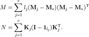
where
The numerator of  can then be written as:
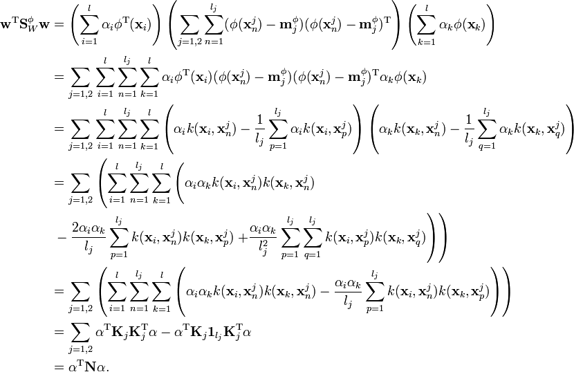
where  . Similarly, the denominator can be written as
where
with the  component of
  defined as
  ,
,  is the identity matrix, and
  the matrix with all entries equal to
  . This identity can be derived by starting out with the expression for
  and using the expansion of
  and the definitions of
  and
and 
With these equations for the numerator and denominator of  , the equation for
  can be rewritten as
Then, differentiating and setting equal to zero gives
Since only the direction of  , and hence the direction of
  , matters, the above can be solved for
  as
as
Note that in practice,  is usually singular and so a multiple of the identity is added to it [1]
Given the solution for  , the projection of a new data point is given by[1]
Multi-class KFD
The extension to cases where there are more than two classes is relatively straightforward.[2][6][7] Let  be the number of classes. Then multi-class KFD involves projecting the data into a
  -dimensional space using
  discriminant functions
This can be written in matrix notation
where the  are the columns of
  .[6] Further, the between-class covariance matrix is now
where  is the mean of all the data in the new feature space. The within-class covariance matrix is
The solution is now obtained by maximizing
The kernel trick can again be used and the goal of multi-class KFD becomes[7]
where ![A = [\mathbf{\alpha}_1,\ldots,\mathbf{\alpha}_{c-1}]](../I/m/2c019510cbf1df8ea63db9156028744f.png) and
and
The  are defined as in the above section and
  is defined as
 can then be computed by finding the
  leading eigenvectors of
  .[7] Furthermore, the projection of a new input,
  , is given by[7]
where the  component of
  is given by
  .
.
Classification using KFD
In both two-class and multi-class KFD, the class label of a new input can be assigned as[7]
where  is the projected mean for class
  and
and  is a distance function.
Applications
Kernel discriminant analysis has been used in a variety of applications. These include:
- Face recognition[3][8][9] and detection[10][11]
- Hand-written digit recognition[1][12]
- Palmprint recognition[13]
- Classification of malignant and benign cluster microcalcifications[14]
- Seed classification[2]
See also
References
- 1 2 3 4 5 Mika, S; Rätsch, G.; Weston, J.; Schölkopf, B.; Müller, KR (1999). "Fisher discriminant analysis with kernels". Neural Networks for Signal Processing IX: 41–48. doi:10.1109/NNSP.1999.788121.
- 1 2 3 Baudat, G.; Anouar, F. (2000). "Generalized discriminant analysis using a kernel approach". Neural Computation 12 (10): 2385–2404. doi:10.1162/089976600300014980.
- 1 2 Li, Y.; Gong, S.; Liddell, H. (2003). "Recognising trajectories of facial identities using kernel discriminant analysis". Image and Vision Computing 21 (13-14): 1077–1086. doi:10.1016/j.imavis.2003.08.010.
- ↑ Bishop, CM (2006). Pattern Recognition and Machine Learning. New York, NY: Springer.
- ↑ Scholkopf, B; Herbrich, R.; Smola, A. (2001). "A generalized representer theorem". Computational learning theory.
- 1 2 Duda, R.; Hart, P.; Stork, D. (2001). Pattern Classification. New York, NY: Wiley.
- 1 2 3 4 5 Zhang, J.; Ma, K.K. (2004). "Kernel fisher discriminant for texture classification".
- ↑ Liu, Q.; Lu, H.; Ma, S. (2004). "Improving kernel Fisher discriminant analysis for face recognition". IEEE Transactions on Circuits and Systems for Video Technology 14 (1): 42–49. doi:10.1109/tcsvt.2003.818352.
- ↑ Liu, Q.; Huang, R.; Lu, H.; Ma, S. (2002). "Face recognition using kernel-based Fisher discriminant analysis". IEEE International Conference on Automatic Face and Gesture Recognition.
- ↑ Kurita, T.; Taguchi, T. (2002). "A modification of kernel-based Fisher discriminant analysis for face detection". IEEE International Conference on Automatic Face and Gesture Recognition.
- ↑ Feng, Y.; Shi, P. (2004). "Face detection based on kernel fisher discriminant analysis". IEEE International Conference on Automatic Face and Gesture Recognition.
- ↑ Yang, J.; Frangi, AF; Yang, JY; Zang, D., Jin, Z. (2005). "KPCA plus LDA: a complete kernel Fisher discriminant framework for feature extraction and recognition". IEEE Transactions on Pattern Analysis and Machine Intelligence 27 (2). doi:10.1109/tpami.2005.33.
- ↑ Wang, Y.; Ruan, Q. (2006). "Kernel fisher discriminant analysis for palmprint recognition". International Conference on Pattern Recognition.
- ↑ Wei, L.; Yang, Y.; Nishikawa, R.M.; Jiang, Y. (2005). "A study on several machine-learning methods for classification of malignant and benign clustered microcalcifications". IEEE Transactions on Medical Imaging 24 (3): 371–380. doi:10.1109/tmi.2004.842457.
External links
- Kernel Discriminant Analysis in C# - C# code to perform KFD.
- Matlab Toolbox for Dimensionality Reduction - Includes a method for performing KFD.
- Handwriting Recognition using Kernel Discriminant Analysis - C# code that demonstrates handwritten digit recognition using KFD.


