Kernel (image processing)

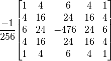
In image processing, a kernel, convolution matrix, or mask is a small matrix useful for blurring, sharpening, embossing, edge-detection, and more. This is accomplished by means of convolution between a kernel and an image.

Details

Depending on the element values, a kernel can cause a wide range of effects.

Identity	$\begin{bmatrix} 0 & 0 & 0 \\ 0 & 1 & 0 \\ 0 & 0 & 0 \end{bmatrix}$
Edge detection	$\begin{bmatrix} \ \ 1 & 0 & -1 \\ \ \ 0 & 0 & \ \ 0 \\ -1 & 0 & \ \ 1 \end{bmatrix}$
	$\begin{bmatrix} 0 & \ \ 1 & 0 \\ 1 & -4 & 1 \\ 0 & \ \ 1 & 0 \end{bmatrix}$
	$\begin{bmatrix} -1 & -1 & -1 \\ -1 & \ \ 8 & -1 \\ -1 & -1 & -1 \end{bmatrix}$
Sharpen	$\begin{bmatrix} \ \ 0 & -1 & \ \ 0 \\ -1 & \ \ 5 & -1 \\ \ \ 0 & -1 & \ \ 0 \end{bmatrix}$
Box blur (normalized)	$\frac{1}{9} \begin{bmatrix} 1 & 1 & 1 \\ 1 & 1 & 1 \\ 1 & 1 & 1 \end{bmatrix}$
Gaussian blur (approximation)	$\frac{1}{16} \begin{bmatrix} 1 & 2 & 1 \\ 2 & 4 & 2 \\ 1 & 2 & 1 \end{bmatrix}$
5×5 Unsharp (with no image mask)	$\frac{-1}{256} \begin{bmatrix} 1 & 4 & \ \ 6 & 4 & 1 \\ 4 & 16 & \ \ 24 & 16 & 4 \\ 6 & 24 & -476 & 24 & 6 \\ 4 & 16 & \ \ 24 & 16 & 4 \\ 1 & 4 & \ \ 6 & 4 & 1 \end{bmatrix}$

The above are just a few examples of effects achievable by convolving kernels and images.

Origin

The origin is the position of the kernel which is above (conceptually) the current output pixel. This could be outside of the actual kernel, though usually it corresponds to one of the kernel elements. For a symmetric kernel, the origin is usually the center element.

Convolution

This is loosely related to a form of mathematical convolution. It should be noted that the matrix operation being performed - convolution - is not traditional matrix multiplication, despite being similarly denoted by *. In words convolution is: given two three-by-three matrices, one a kernel, and the other an image piece, convolution is the process of multiplying locationaly similar entries and summing: $\begin{bmatrix} a & b & c \\ d & e & f \\ g & h & i \end{bmatrix} * \begin{bmatrix} 1 & 2 & 3 \\ 4 & 5 & 6 \\ 7 & 8 & 9 \end{bmatrix} = (1*i)+(2*h)+(3*g)+(4*f)+(5*e)+(6*d)+(7*c)+(8*b)+(9*a)$ .

The values of a given pixel in the output image are calculated by multiplying each kernel value by the corresponding input image pixel values. This can be described algorithmically with the following pseudo-code:

for each image row in input image:
   for each pixel in image row:

      set accumulator to zero

      for each kernel row in kernel:
         for each element in kernel row:

            if element position  corresponding* to pixel position then
               multiply element value  corresponding* to pixel value
               add result to accumulator
            endif

      set output image pixel to accumulator

*corresponding input image pixels are found relative to the kernel's origin.

If kernel is symmetric then place the centre(origin) of kernel on the current pixel. Then kernel will be overlapped with neighboring pixels too. Now multiply each kernel element with the pixel value it overlapped with and add all the obtained values. Resultant value will be the value for the current pixel that is overlapped with the center of the kernel.

If the kernel is not symmetric, it has to be flipped both around its horizontal and vertical axis before calculating the convolution as above.^[1]

Edge Handling

Extend Edge-Handling

Kernel convolution usually requires values from pixels outside of the image boundaries. There are a variety of methods for handling image edges.

Extend: The nearest border pixels are conceptually extended as far as necessary to provide values for the convolution. Corner pixels are extended in 90° wedges. Other edge pixels are extended in lines.
Wrap: The image is conceptually wrapped (or tiled) and values are taken from the opposite edge or corner.
Crop: Any pixel in the output image which would require values from beyond the edge is skipped. This method can result in the output image being slightly smaller, with the edges having been cropped.

Normalization

Dividing each element in the kernel by the sum of all the absolute values of the elements in the kernel. Normalization ensures that the pixel values in the output image are of the same relative magnitude as those in the input image.

References

↑ http://www.songho.ca/dsp/convolution/convolution2d_example.html

Ludwig, Jamie (n.d.). Image Convolution (pdf). Portland State University.
Lecarme, Olivier; Delvare, Karine (January 2013). The Book of GIMP: A Complete Guide to Nearly Everything. No Starch Press. p. 429. ISBN 978-1593273835.
Gumster, Jason van; Shimonski, Robert (March 2012). GIMP Bible. Wiley. pp. 438–442. ISBN 978-0470523971.
Stockman, George C.; Shapiro, Linda G. (February 2001). Computer Vision. Prentice Hall. pp. 53–54. ISBN 978-0130307965.

External links

This article is issued from Wikipedia - version of the Monday, February 08, 2016. The text is available under the Creative Commons Attribution/Share Alike but additional terms may apply for the media files.