Interferometry

Figure 1. The light path through a Michelson interferometer. The two light rays with a common source combine at the half-silvered mirror to reach the detector. They may either interfere constructively (strengthening in intensity) if their light waves arrive in phase, or interfere destructively (weakening in intensity) if they arrive out of phase, depending on the exact distances between the three mirrors.

Interferometry is a family of techniques in which waves, usually electromagnetic, are superimposed in order to extract information about the waves.^[1] Interferometry is an important investigative technique in the fields of astronomy, fiber optics, engineering metrology, optical metrology, oceanography, seismology, spectroscopy (and its applications to chemistry), quantum mechanics, nuclear and particle physics, plasma physics, remote sensing, biomolecular interactions, surface profiling, microfluidics, mechanical stress/strain measurement, and velocimetry.^[2]:1–2

Interferometers are widely used in science and industry for the measurement of small displacements, refractive index changes and surface irregularities. In analytical science, interferometers are used in continuous wave Fourier transform spectroscopy to analyze light containing features of absorption or emission associated with a substance or mixture. An astronomical interferometer consists of two or more separate telescopes that combine their signals, offering a resolution equivalent to that of a telescope of diameter equal to the largest separation between its individual elements.

Basic principles

Figure 2. Formation of fringes in a Michelson interferometer

Figure 3. Colored and monochromatic fringes in a Michelson interferometer: (a) White light fringes where the two beams differ in the number of phase inversions; (b) White light fringes where the two beams have experienced the same number of phase inversions; (c) Fringe pattern using monochromatic light (sodium D lines)

Interferometry makes use of the principle of superposition to combine waves in a way that will cause the result of their combination to have some meaningful property that is diagnostic of the original state of the waves. This works because when two waves with the same frequency combine, the resulting pattern is determined by the phase difference between the two waves—waves that are in phase will undergo constructive interference while waves that are out of phase will undergo destructive interference. Most interferometers use light or some other form of electromagnetic wave.^[2]:3–12

Typically (see Fig. 1, the well-known Michelson configuration) a single incoming beam of coherent light will be split into two identical beams by a beam splitter (a partially reflecting mirror). Each of these beams travels a different route, called a path, and they are recombined before arriving at a detector. The path difference, the difference in the distance traveled by each beam, creates a phase difference between them. It is this introduced phase difference that creates the interference pattern between the initially identical waves.^[2]:14–17 If a single beam has been split along two paths, then the phase difference is diagnostic of anything that changes the phase along the paths. This could be a physical change in the path length itself or a change in the refractive index along the path.^[2]:93–103

As seen in Fig. 2a and 2b, the observer has a direct view of mirror M₁ seen through the beam splitter, and sees a reflected image M'₂ of mirror M₂. The fringes can be interpreted as the result of interference between light coming from the two virtual images S'₁ and S'₂ of the original source S. The characteristics of the interference pattern depend on the nature of the light source and the precise orientation of the mirrors and beam splitter. In Fig. 2a, the optical elements are oriented so that S'₁ and S'₂ are in line with the observer, and the resulting interference pattern consists of circles centered on the normal to M₁ and M'₂. If, as in Fig. 2b, M₁ and M'₂ are tilted with respect to each other, the interference fringes will generally take the shape of conic sections (hyperbolas), but if M₁ and M'₂ overlap, the fringes near the axis will be straight, parallel, and equally spaced. If S is an extended source rather than a point source as illustrated, the fringes of Fig. 2a must be observed with a telescope set at infinity, while the fringes of Fig. 2b will be localized on the mirrors.^[2]:17

Use of white light will result in a pattern of colored fringes (see Fig. 3).^[2]:26 The central fringe representing equal path length may be light or dark depending on the number of phase inversions experienced by the two beams as they traverse the optical system.^{[2]:26,171–172} (See Michelson interferometer for a discussion of this.)

Categories

Interferometers and interferometric techniques may be categorized by a variety of criteria:

Homodyne versus heterodyne detection

• In homodyne detection, the interference occurs between two beams at the same wavelength (or carrier frequency). The phase difference between the two beams results in a change in the intensity of the light on the detector. The resulting intensity of the light after mixing of these two beams is measured, or the pattern of interference fringes is viewed or recorded.^[3] Most of the interferometers discussed in this article fall into this category.
• The heterodyne technique is used for (1) shifting an input signal into a new frequency range as well as (2) amplifying a weak input signal (assuming use of an active mixer). A weak input signal of frequency f₁ is mixed with a strong reference frequency f₂ from a local oscillator (LO). The nonlinear combination of the input signals creates two new signals, one at the sum f₁ + f₂ of the two frequencies, and the other at the difference f₁ − f₂. These new frequencies are called heterodynes. Typically only one of the new frequencies is desired, and the other signal is filtered out of the output of the mixer. The output signal will have an intensity proportional to the product of the amplitudes of the input signals.^[3]

The most important and widely used application of the heterodyne technique is in the superheterodyne receiver (superhet), invented by U.S. engineer Edwin Howard Armstrong in 1918. In this circuit, the incoming radio frequency signal from the antenna is mixed with a signal from a local oscillator (LO) and converted by the heterodyne technique to a lower fixed frequency signal called the intermediate frequency (IF). This IF is amplified and filtered, before being applied to a detector which extracts the audio signal, which is sent to the loudspeaker.^[4]

Optical heterodyne detection is an extension of the heterodyne technique to higher (visible) frequencies.^[3]

Double path versus common path

• A double path interferometer is one in which the reference beam and sample beam travel along divergent paths. Examples include the Michelson interferometer, the Twyman-Green interferometer, and the Mach-Zehnder interferometer. After being perturbed by interaction with the sample under test, the sample beam is recombined with the reference beam to create an interference pattern which can then be interpreted.^[2]:13–22
• A common path interferometer is a class of interferometer in which the reference beam and sample beam travel along the same path. Fig. 4 illustrates the Sagnac interferometer, the fibre optic gyroscope, the point diffraction interferometer, and the lateral shearing interferometer. Other examples of common path interferometer include the Zernike phase contrast microscope, Fresnel's biprism, the zero-area Sagnac, and the scatterplate interferometer.^[5]

Figure 4. Four examples of common path interferometers

Wavefront splitting versus amplitude splitting

• A wavefront splitting interferometer divides a light wavefront emerging from a point or a narrow slit (i.e. spatially coherent light) and, after allowing the two parts of the wavefront to travel through different paths, allows them to recombine.^[6] Fig. 5 illustrates Young's interference experiment and Lloyd's mirror. Other examples of wavefront splitting interferometer include the Fresnel biprism, the Billet Bi-Lens, and the Rayleigh interferometer.^[7]

Figure 5. Two wavefront splitting interferometers

• In 1803, Young's interference experiment played a major role in the general acceptance of the wave theory of light. If white light is used in Young's experiment, the result is a white central band of constructive interference corresponding to equal path length from the two slits, surrounded by a symmetrical pattern of colored fringes of diminishing intensity. In addition to continuous electromagnetic radiation, Young's experiment has been performed with individual photons,^[8] with electrons,^[9][10] and with buckyball molecules large enough to be seen under an electron microscope.^[11]
• Lloyd's mirror generates interference fringes by combining direct light from a source (blue lines) and light from the source's reflected image (red lines) from a mirror held at grazing incidence. The result is an asymmetrical pattern of fringes. Interestingly, the band of equal path length, nearest the mirror, is dark rather than bright. In 1834, Humphrey Lloyd interpreted this effect as proof that the phase of a front-surface reflected beam is inverted.^[12][13]

• An amplitude splitting interferometer uses a partial reflector to divide the amplitude of the incident wave into separate beams which are separated and recombined. Fig. 6 illustrates the Fizeau, Mach–Zehnder and Fabry–Pérot interferometers. Other examples of amplitude splitting interferometer include the Michelson, Twyman–Green, Laser Unequal Path, and Linnik interferometer.^[14]

Figure 6. Three amplitude-splitting interferometers: Fizeau, Mach–Zehnder, and Fabry Pérot

• The Fizeau interferometer is shown as it might be set up to test an optical flat. A precisely figured reference flat is placed on top of the flat being tested, separated by narrow spacers. The reference flat is slightly beveled (only a fraction of a degree of beveling is necessary) to prevent the rear surface of the flat from producing interference fringes. Separating the test and reference flats allows the two flats to be tilted with respect to each other. By adjusting the tilt, which adds a controlled phase gradient to the fringe pattern, one can control the spacing and direction of the fringes, so that one may obtain an easily interpreted series of nearly parallel fringes rather than a complex swirl of contour lines. Separating the plates, however, necessitates that the illuminating light be collimated. Fig 6 shows a collimated beam of monochromatic light illuminating the two flats and a beam splitter allowing the fringes to be viewed on-axis.^[15][16]
• The Mach–Zehnder interferometer is a more versatile instrument than the Michelson interferometer. Each of the well separated light paths is traversed only once, and the fringes can be adjusted so that they are localized in any desired plane.^[2]:18 Typically, the fringes would be adjusted to lie in the same plane as the test object, so that fringes and test object can be photographed together. If it is decided to produce fringes in white light, then, since white light has a limited coherence length, on the order of micrometers, great care must be taken to equalize the optical paths or no fringes will be visible. As illustrated in Fig. 6, a compensating cell would be placed in the path of the reference beam to match the test cell. Note also the precise orientation of the beam splitters. The reflecting surfaces of the beam splitters would be oriented so that the test and reference beams pass through an equal amount of glass. In this orientation, the test and reference beams each experience two front-surface reflections, resulting in the same number of phase inversions. The result is that light traveling an equal optical path length in the test and reference beams produces a white light fringe of constructive interference.^[17][18]
• The heart of the Fabry–Pérot interferometer is a pair of partially silvered glass optical flats spaced several millimeters to centimeters apart with the silvered surfaces facing each other. (Alternatively, a Fabry–Pérot etalon uses a transparent plate with two parallel reflecting surfaces.)^[2]:35–36 As with the Fizeau interferometer, the flats are slightly beveled. In a typical system, illumination is provided by a diffuse source set at the focal plane of a collimating lens. A focusing lens produces what would be an inverted image of the source if the paired flats were not present; i.e. in the absence of the paired flats, all light emitted from point A passing through the optical system would be focused at point A'. In Fig. 6, only one ray emitted from point A on the source is traced. As the ray passes through the paired flats, it is multiply reflected to produce multiple transmitted rays which are collected by the focusing lens and brought to point A' on the screen. The complete interference pattern takes the appearance of a set of concentric rings. The sharpness of the rings depends on the reflectivity of the flats. If the reflectivity is high, resulting in a high Q factor (i.e. high finesse), monochromatic light produces a set of narrow bright rings against a dark background.^[19] In Fig. 6, the low-finesse image corresponds to a reflectivity of 0.04 (i.e. unsilvered surfaces) versus a reflectivity of 0.95 for the high-finesse image.

• It is interesting to note that Michelson and Morley (1887)^[20] and other early experimentalists using interferometric techniques in an attempt to measure the properties of the luminiferous aether, used monochromatic light only for initially setting up their equipment, always switching to white light for the actual measurements. The reason is that measurements were recorded visually. Monochromatic light would result in a uniform fringe pattern. Lacking modern means of environmental temperature control, experimentalists struggled with continual fringe drift even though the interferometer might be set up in a basement. Since the fringes would occasionally disappear due to vibrations by passing horse traffic, distant thunderstorms and the like, it would be easy for an observer to "get lost" when the fringes returned to visibility. The advantages of white light, which produced a distinctive colored fringe pattern, far outweighed the difficulties of aligning the apparatus due to its low coherence length.^[21] This was an early example of the use of white light to resolve the "2 pi ambiguity".

Applications

Physics and astronomy

• In physics, one of the most important experiments of the late 19th century was the famous "failed experiment" of Michelson and Morley which provided evidence for special relativity. Recent repetitions of the Michelson–Morley experiment perform heterodyne measurements of beat frequencies of crossed cryogenic optical resonators. Fig 7 illustrates a resonator experiment performed by Müller et al. in 2003.^[22] Two optical resonators constructed from crystalline sapphire, controlling the frequencies of two lasers, were set at right angles within a helium cryostat. A frequency comparator measured the beat frequency of the combined outputs of the two resonators. As of 2009, the precision by which anisotropy of the speed of light can be excluded in resonator experiments is at the 10⁻¹⁷ level.^[23][24]

Figure 7. Michelson-Morley experiment with cryogenic optical resonators

Figure 8. Fourier transform spectroscopy

Figure 9. A picture of the solar corona taken with the LASCO C1 coronagraph

Michelson interferometers are used in tunable narrow band optical filters^[25] and as the core hardware component of Fourier transform spectrometers.^[26]

When used as a tunable narrow band filter, Michelson interferometers exhibit a number of advantages and disadvantages when compared with competing technologies such as Fabry–Pérot interferometers or Lyot filters. Michelson interferometers have the largest field of view for a specified wavelength, and are relatively simple in operation, since tuning is via mechanical rotation of waveplates rather than via high voltage control of piezoelectric crystals or lithium niobate optical modulators as used in a Fabry–Pérot system. Compared with Lyot filters, which use birefringent elements, Michelson interferometers have a relatively low temperature sensitivity. On the negative side, Michelson interferometers have a relatively restricted wavelength range and require use of prefilters which restrict transmittance.^[27]

Fig. 8 illustrates the operation of a Fourier transform spectrometer, which is essentially a Michelson interferometer with one mirror movable. (A practical Fourier transform spectrometer would substitute corner cube reflectors for the flat mirrors of the conventional Michelson interferometer, but for simplicity, the illustration does not show this.) An interferogram is generated by making measurements of the signal at many discrete positions of the moving mirror. A Fourier transform converts the interferogram into an actual spectrum.^[28]

• Fig. 9 shows a doppler image of the solar corona made using a tunable Fabry-Pérot interferometer to recover scans of the solar corona at a number of wavelengths near the FeXIV green line. The picture is a color-coded image of the doppler shift of the line, which may be associated with the coronal plasma velocity towards or away from the satellite camera.

Fabry-Pérot thin-film etalons are used in narrow bandpass filters capable of selecting a single spectral line for imaging; for example, the H-alpha line or the Ca-K line of the Sun or stars. Fig. 10 shows an Extreme ultraviolet Imaging Telescope (EIT) image of the Sun at 195 Ångströms, corresponding to a spectral line of multiply-ionized iron atoms.^[29] EIT used multilayer coated reflective mirrors that were coated with alternate layers of a light "spacer" element (such as silicon), and a heavy "scatterer" element (such as molybdenum). Approximately 100 layers of each type were placed on each mirror, with a thickness of around 10 nm each. The layer thicknesses were tightly controlled so that at the desired wavelength, reflected photons from each layer interfered constructively.

The Laser Interferometer Gravitational-Wave Observatory (LIGO) uses two 4-km Michelson-Fabry-Pérot interferometers for the detection of gravitational waves.^[30] In this application, the Fabry–Pérot cavity is used to store photons for almost a millisecond while they bounce up and down between the mirrors. This increases the time a gravitational wave can interact with the light, which results in a better sensitivity at low frequencies. Smaller cavities, usually called mode cleaners, are used for spatial filtering and frequency stabilization of the main laser.

• The Mach-Zehnder interferometer's relatively large and freely accessible working space, and its flexibility in locating the fringes has made it the interferometer of choice for visualizing flow in wind tunnels,^[31][32] and for flow visualization studies in general. It is frequently used in the fields of aerodynamics, plasma physics and heat transfer to measure pressure, density, and temperature changes in gases.^{[2]:18,93–95}

Mach-Zehnder interferometers are also used to study one of the most counterintuitive predictions of quantum mechanics, the phenomenon known as quantum entanglement.^[33][34]

Figure 11. The VLA interferometer

• An astronomical interferometer achieves high-resolution observations using the technique of aperture synthesis, mixing signals from a cluster of comparatively small telescopes rather than a single very expensive monolithic telescope.^[35]

Early radio telescope interferometers used a single baseline for measurement. Later astronomical interferometers, such as the Very Large Array illustrated in Fig 11, used arrays of telescopes arranged in a pattern on the ground. A limited number of baselines will result in insufficient coverage. This was alleviated by using the rotation of the Earth to rotate the array relative to the sky. Thus, a single baseline could measure information in multiple orientations by taking repeated measurements, a technique called Earth-rotation synthesis. Baselines thousands of kilometers long were achieved using very long baseline interferometry.^[35]

Astronomical optical interferometry has had to overcome a number of technical issues not shared by radio telescope interferometry. The short wavelengths of light necessitate extreme precision and stability of construction. For example, spatial resolution of 1 milliarcsecond requires 0.5 µm stability in a 100 m baseline. Optical interferometric measurements require high sensitivity, low noise detectors that did not become available until the late 1990s. Astronomical "seeing", the turbulence that causes stars to twinkle, introduces rapid, random phase changes in the incoming light, requiring kilohertz data collection rates to be faster than the rate of turbulence.^[36][37] Despite these technical difficulties, roughly a dozen astronomical optical interferometers are now in operation offering resolutions down to the fractional milliarcsecond range. Fig. 12 shows a movie assembled from aperture sythesis images of the Beta Lyrae system, a binary star system approximately 960 light-years (290 parsecs) away in the constellation Lyra, as observed by the CHARA array with the MIRC instrument. The brighter component is the primary star, or the mass donor. The fainter component is the thick disk surrounding the secondary star, or the mass gainer. The two components are separated by 1 milli-arcsecond. Tidal distortions of the mass donor and the mass gainer are both clearly visible.^[38]

• The wave character of matter can be exploited to build interferometers. The first examples of matter interferometers were electron interferometers, later followed by neutron interferometers. Around 1990 the first atom interferometers were demonstrated, later followed by interferometers employing molecules.^[39]

Electron holography is an imaging technique that photographically records the electron interference pattern of an object, which is then reconstructed to yield a greatly magnified image of the original object.^[40] This technique was developed to enable greater resolution in electron microscopy than is possible using conventional imaging techniques. The resolution of conventional electron microscopy is not limited by electron wavelength, but by the large aberrations of electron lenses.^[41]

Neutron interferometry has been used to investigate the Aharonov–Bohm effect, to examine the effects of gravity acting on an elementary particle, and to demonstrate a strange behavior of fermions that is at the basis of the Pauli exclusion principle: Unlike macroscopic objects, when fermions are rotated by 360° about any axis, they do not return to their original state, but develop a minus sign in their wave function. In other words, a fermion needs to be rotated 720° before returning to its original state.^[42]

Atom interferometry techniques are reaching sufficient precision to allow laboratory-scale tests of general relativity.^[43]

• Interferometers are used in atmospheric physics for high-precision measurements of trace gases via remote sounding of the atmosphere. There are several examples of interferometers that utilize either absorption or emission features of trace gases. A typical use would be in continual monitoring of the column concentration of trace gases such as Ozone and Carbon Monoxide above the instrument.^[44]

Engineering and applied science

Figure 13. Optical flat interference fringes

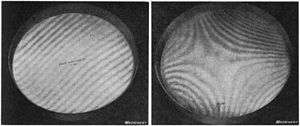
• Newton (test plate) interferometry is frequently used in the optical industry for testing the quality of surfaces as they are being shaped and figured. Fig. 13 shows photos of reference flats being used to check two test flats at different stages of completion, showing the different patterns of interference fringes. The reference flats are resting with their bottom surfaces in contact with the test flats, and they are illuminated by a monochromatic light source. The light waves reflected from both surfaces interfere, resulting in a pattern of bright and dark bands. The surface in the left photo is nearly flat, indicated by a pattern of straight parallel interference fringes at equal intervals. The surface in the right photo is uneven, resulting in a pattern of curved fringes. Each pair of adjacent fringes represents a difference in surface elevation of half a wavelength of the light used, so differences in elevation can be measured by counting the fringes. The flatness of the surfaces can be measured to millionths of an inch by this method. To determine whether the surface being tested is concave or convex with respect to the reference optical flat, any of several procedures may be adopted. One can observe how the fringes are displaced when one presses gently on the top flat. If one observes the fringes in white light, the sequence of colors becomes familiar with experience and aids in interpretation. Finally one may compare the appearance of the fringes as one moves ones head from a normal to an oblique viewing position.^[45] These sorts of maneuvers, while common in the optical shop, are not suitable in a formal testing environment. When the flats are ready for sale, they will typically be mounted in a Fizeau interferometer for formal testing and certification.
• Fabry-Pérot etalons are widely used in telecommunications, lasers and spectroscopy to control and measure the wavelengths of light. Dichroic filters are multiple layer thin-film etalons. In telecommunications, wavelength-division multiplexing, the technology that enables the use of multiple wavelengths of light through a single optical fiber, depends on filtering devices that are thin-film etalons. Single-mode lasers employ etalons to suppress all optical cavity modes except the single one of interest.^[2]:42

Figure 14. Twyman-Green Interferometer

• The Twyman–Green interferometer, invented by Twyman and Green in 1916, is a variant of the Michelson interferometer widely used to test optical components.^[46] The basic characteristics distinguishing it from the Michelson configuration are the use of a monochromatic point light source and a collimator. It is interesting to note that Michelson (1918) criticized the Twyman-Green configuration as being unsuitable for the testing of large optical components, since the light sources available at the time had limited coherence length. Michelson pointed out that constraints on geometry forced by limited coherence length required the use of a reference mirror of equal size to the test mirror, making the Twyman-Green impractical for many purposes.^[47] Decades later, the advent of laser light sources answered Michelson's objections. (A Twyman-Green interferometer using a laser light source and unequal path length is known as a Laser Unequal Path Interferometer, or LUPI.) Fig. 14 illustrates a Twyman-Green interferometer set up to test a lens. Light from a monochromatic point source is expanded by a diverging lens (not shown), then is collimated into a parallel beam. A convex spherical mirror is positioned so that its center of curvature coincides with the focus of the lens being tested. The emergent beam is recorded by an imaging system for analysis.^[48]
• Mach-Zehnder interferometers are being used in integrated optical circuits, in which light interferes between two branches of a waveguide that are externally modulated to vary their relative phase. A slight tilt of one of the beam splitters will result in a path difference and a change in the interference pattern. Mach-Zehnder interferometers are the basis of a wide variety of devices, from RF modulators to sensors^[49][50] to optical switches.^[51]
• The latest proposed extremely large astronomical telescopes, such as the Thirty Meter Telescope and the European Extremely Large Telescope, will be of segmented design. Their primary mirrors will be built from hundreds of hexagonal mirror segments. Polishing and figuring these highly aspheric and non-rotationally symmetric mirror segments presents a major challenge. Traditional means of optical testing compares a surface against a spherical reference with the aid of a null corrector. In recent years, computer-generated holograms (CGHs) have begun to supplement null correctors in test setups for complex aspheric surfaces. Fig. 15 illustrates how this is done. Unlike the figure, actual CGHs have line spacing on the order of 1 to 10 µm. When laser light is passed through the CGH, the zero-order diffracted beam experiences no wavefront modification. The wavefront of the first-order diffracted beam, however, is modified to match the desired shape of the test surface. In the illustrated Fizeau interferometer test setup, the zero-order diffracted beam is directed towards the spherical reference surface, and the first-order diffracted beam is directed towards the test surface in such a way that the two reflected beams combine to form interference fringes. The same test setup can be used for the innermost mirrors as for the outermost, with only the CGH needing to be exchanged.^[52]

Figure 15. Optical testing with a Fizeau interferometer and a computer generated hologram

• Ring laser gyroscopes (RLGs) and fibre optic gyroscopes (FOGs) are interferometers used in navigation systems. They operate on the principle of the Sagnac effect. The distinction between RLGs and FOGs is that in a RLG, the entire ring is part of the laser while in a FOG, an external laser injects counter-propagating beams into an optical fiber ring, and rotation of the system then causes a relative phase shift between those beams. In a RLG, the observed phase shift is proportional to the accumulated rotation, while in a FOG, the observed phase shift is proportional to the angular velocity.^[53]
• In telecommunication networks, heterodyning is used to move frequencies of individual signals to different channels which may share a single physical transmission line. This is called frequency division multiplexing (FDM). For example, a coaxial cable used by a cable television system can carry 500 television channels at the same time because each one is given a different frequency, so they don't interfere with one another. Continuous wave (CW) doppler radar detectors are basically heterodyne detection devices that compare transmitted and reflected beams.^[54]

Optical heterodyne detection is used for coherent Doppler lidar measurements capable of detecting very weak light scattered in the atmosphere and monitoring wind speeds with high accuracy. It has application in optical fiber communications, in various high resolution spectroscopic techniques, and the self-heterodyne method can be used to measure the linewidth of a laser.^[3][55]

Figure 16. Frequency comb of a mode-locked laser. The dashed lines represent an extrapolation of the mode frequencies towards the frequency of the carrier–envelope offset (CEO). The vertical grey line represents an unknown optical frequency. The horizontal black lines indicate the two lowest beat frequency measurements.

Optical heterodyne detection is an essential technique used in high-accuracy measurements of the frequencies of optical sources, as well as in the stabilization of their frequencies. Until a relatively few years ago, lengthy frequency chains were needed to connect the microwave frequency of a cesium or other atomic time source to optical frequencies. At each step of the chain, a frequency multiplier would be used to produce a harmonic of the frequency of that step, which would be compared by heterodyne detection with the next step (the output of a microwave source, far infrared laser, infrared laser, or visible laser). Each measurement of a single spectral line required several years of effort in the construction of a custom frequency chain. Currently, optical frequency combs have provided a much simpler method of measuring optical frequencies. If a mode-locked laser is modulated to form a train of pulses, its spectrum is seen to consist of the carrier frequency surrounded by a closely spaced comb of optical sideband frequencies with a spacing equal to the pulse repetition frequency (Fig. 16). The pulse repetition frequency is locked to that of the frequency standard, and the frequencies of the comb elements at the red end of the spectrum are doubled and heterodyned with the frequencies of the comb elements at the blue end of the spectrum, thus allowing the comb to serve as its own reference. In this manner, locking of the frequency comb output to an atomic standard can be performed in a single step. To measure an unknown frequency, the frequency comb output is dispersed into a spectrum. The unknown frequency is overlapped with the appropriate spectral segment of the comb and the frequency of the resultant heterodyne beats is measured.^[56][57]

• One of the most common industrial applications of optical interferometry is as a versatile measurement tool for the high precision examination of surface topography. Popular interferometric measurement techniques include Phase Shifting Interferometry (PSI),^[58] and Vertical Scanning Interferometry(VSI),^[59] also known as scanning white light interferometry (SWLI) or by the ISO term Coherence Scanning Interferometry (CSI),^[60] CSI exploits coherence to extend the range of capabilities for interference microscopy.^[61][62] These techniques are widely used in micro-electronic and micro-optic fabrication. PSI uses monochromatic light and provides very precise measurements; however it is only usable for surfaces that are very smooth. CSI often uses white light and high numerical apertures, and rather than looking at the phase of the fringes, as does PSI, looks for best position of maximum fringe contrast or some other feature of the overall fringe pattern. In its simplest form, CSI provides less precise measurements than PSI but can be used on rough surfaces. Some configurations of CSI, variously known as and Enhanced VSI (EVSI), high-resolution SWLI or Frequency Domain Analysis (FDA), use coherence effects in combination with interference phase to enhance precision.^[63][64]

Figure 17. Phase shifting and Coherence scanning interferometers

• Phase Shifting Interferometry addresses several issues associated with the classical analysis of static interferograms. Classically, one measures the positions of the fringe centers. As seen in Fig. 13, fringe deviations from straightness and equal spacing provide a measure of the aberration. Errors in determining the location of the fringe centers provide the inherent limit to precision of the classical analysis, and any intensity variations across the interferogram will also introduce error. There is a trade-off between precision and number of data points: closely spaced fringes provide many data points of low precision, while widely spaced fringes provide a low number of high precision data points. Since fringe center data is all that one uses in the classical analysis, all of the other information that might theoretically be obtained by detailed analysis of the intensity variations in an interferogram is thrown away.^[65][66] Finally, with static interferograms, additional information is needed to determine the polarity of the wavefront: In Fig. 13, one can see that the tested surface on the right deviates from flatness, but one cannot tell from this single image whether this deviation from flatness is concave or convex. Traditionally, this information would be obtained using non-automated means, such as by observing the direction that the fringes move when the reference surface is pushed.^[67]

Phase shifting interferometry overcomes these limitations by not relying on finding fringe centers, but rather by collecting intensity data from every point of the CCD image sensor. As seen in Fig. 17, multiple interferograms (at least three) are analyzed with the reference optical surface shifted by a precise fraction of a wavelength between each exposure using a piezoelectric transducer (PZT). Alternatively, precise phase shifts can be introduced by modulating the laser frequency.^[68] The captured images are processed by a computer to calculate the optical wavefront errors. The precision and reproducibility of PSI is far greater than possible in static interferogram analysis, with measurement repeatabilities of a hundredth of a wavelength being routine.^[65][66] Phase shifting technology has been adapted to a variety of interferometer types such as Twyman-Green, Mach–Zehnder, laser Fizeau, and even common path configurations such as point diffraction and lateral shearing interferometers.^[67][69] More generally, phase shifting techniques can be adapted to almost any system that uses fringes for measurement, such as holographic and speckle interferometry.^[67]

Figure 18. Lunate cells of Nepenthes khasiana visualized by Scanning White Light Interferometry (SWLI)

Figure 19. Twyman-Green interferometer set up as a white light scanner

• In coherence scanning interferometry,^[70] interference is only achieved when the path length delays of the interferometer are matched within the coherence time of the light source. CSI monitors the fringe contrast rather than the phase of the fringes.^[2]:105

Fig. 17 illustrates a CSI microscope using a Mirau interferometer in the objective; other forms of interferometer used with white light include the Michelson interferometer (for low magnification objectives, where the reference mirror in a Mirau objective would interrupt too much of the aperture) and the Linnik interferometer (for high magnification objectives with limited working distance).^[71] The sample (or alternatively, the objective) is moved vertically over the full height range of the sample, and the position of maximum fringe contrast is found for each pixel.^[61][72] The chief benefit of coherence scanning interferometry is that systems can be designed that do not suffer from the 2 pi ambiguity of coherent interferometry,^[73][74][75] and as seen in Fig. 18, which scans a 180μm x 140μm x 10μm volume, it is well suited to profiling steps and rough surfaces. The axial resolution of the system is determined in part by the coherence length of the light source.^[76][77] Industrial applications include in-process surface metrology, roughness measurement, 3D surface metrology in hard-to-reach spaces and in hostile environments, profilometry of surfaces with high aspect ratio features (grooves, channels, holes), and film thickness measurement (semi-conductor and optical industries, etc.).^[78][79]

Fig. 19 illustrates a Twyman–Green interferometer set up for white light scanning of a macroscopic object.

• Holographic interferometry is a technique which uses holography to monitor small deformations in single wavelength implementations. In multi-wavelength implementations, it is used to perform dimensional metrology of large parts and assemblies and to detect larger surface defects.^{[2]:111–120}

Holographic interferometry was discovered by accident as a result of mistakes committed during the making of holograms. Early lasers were relatively weak and photographic plates were insensitive, necessitating long exposures during which vibrations or minute shifts might occur in the optical system. The resultant holograms, which showed the holographic subject covered with fringes, were considered ruined.^[80]

Eventually, several independent groups of experimenters in the mid-60s realized that the fringes encoded important information about dimensional changes occurring in the subject, and began intentionally producing holographic double exposures. The main Holographic interferometry article covers the disputes over priority of discovery that occurred during the issuance of the patent for this method.^[81]

Double- and multi- exposure holography is one of three methods used to create holographic interferograms. A first exposure records the object in an unstressed state. Subsequent exposures on the same photographic plate are made while the object is subjected to some stress. The composite image depicts the difference between the stressed and unstressed states.^[82]

Real-time holography is a second method of creating holographic interferograms. A holograph of the unstressed object is created. This holograph is illuminated with a reference beam to generate a hologram image of the object directly superimposed over the original object itself while the object is being subjected to some stress. The object waves from this hologram image will interfere with new waves coming from the object. This technique allows real time monitoring of shape changes.^[82]

The third method, time-average holography, involves creating a holograph while the object is subjected to a periodic stress or vibration. This yields a visual image of the vibration pattern.^[82]

• 

  Figure 20. InSAR Image of Kilauea, Hawaii showing fringes caused by deformation of the terrain over a six-month period.

• 

  Figure 21. ESPI fringes showing a vibration mode of a clamped square plate

• Interferometric synthetic aperture radar (InSAR) is a radar technique used in geodesy and remote sensing. Satellite synthetic aperture radar images of a geographic feature are taken on separate days, and changes that have taken place between radar images taken on the separate days are recorded as fringes similar to those obtained in holographic interferometry. The technique can monitor centimeter- to millimeter-scale deformation resulting from earthquakes, volcanoes and landslides, and also has uses in structural engineering, in particular for the monitoring of subsidence and structural stability. Fig 20 shows Kilauea, an active volcano in Hawaii. Data acquired using the space shuttle Endeavour's X-band Synthetic Aperture Radar on April 13, 1994 and October 4, 1994 were used to generate interferometric fringes, which were overlaid on the X-SAR image of Kilauea.^[83]
• Electronic speckle pattern interferometry (ESPI), also known as TV holography, uses video detection and recording to produce an image of the object upon which is superimposed a fringe pattern which represents the displacement of the object between recordings. (see Fig. 21) The fringes are similar to those obtained in holographic interferometry.^{[2]:111–120[84]}

When lasers were first invented, laser speckle was considered to be a severe drawback in using lasers to illuminate objects, particularly in holographic imaging because of the grainy image produced. It was later realized that speckle patterns could carry information about the object's surface deformations. Butters and Leendertz developed the technique of speckle pattern interferometry in 1970,^[85] and since then, speckle has been exploited in a variety of other applications. A photograph is made of the speckle pattern before deformation, and a second photograph is made of the speckle pattern after deformation. Digital subtraction of the two images results in a correlation fringe pattern, where the fringes represent lines of equal deformation. Short laser pulses in the nanosecond range can be used to capture very fast transient events. A phase problem exists: In the absence of other information, one cannot tell the difference between contour lines indicating a peak versus contour lines indicating a trough. To resolve the issue of phase ambiguity, ESPI may be combined with phase shifting methods.^[86][87]

• A method of establishing precise geodetic baselines, invented by Yrjö Väisälä, exploited the low coherence length of white light. Initially, white light was split in two, with the reference beam "folded", bouncing back-and-forth six times between a mirror pair spaced precisely 1 m apart. Only if the test path was precisely 6 times the reference path would fringes be seen. Repeated applications of this procedure allowed precise measurement of distances up to 864 meters. Baselines thus established were used to calibrate geodetic distance measurement equipment, leading to a metrologically traceable scale for geodetic networks measured by these instruments.^[88] (This method has been superseded by GPS.)
• Other uses of interferometers have been to study dispersion of materials, measurement of complex indices of refraction, and thermal properties. They are also used for three-dimensional motion mapping including mapping vibrational patterns of structures.^[63]

Biology and medicine

Figure 22. Typical optical setup of single point OCT

Figure 23. Central serous retinopathy,imaged using optical coherence tomography

• Optical coherence tomography (OCT) is a medical imaging technique using low-coherence interferometry to provide tomographic visualization of internal tissue microstructures. As seen in Fig. 22, the core of a typical OCT system is a Michelson interferometer. One interferometer arm is focused onto the tissue sample and scans the sample in an X-Y longitudinal raster pattern. The other interferometer arm is bounced off a reference mirror. Reflected light from the tissue sample is combined with reflected light from the reference. Because of the low coherence of the light source, interferometric signal is observed only over a limited depth of sample. X-Y scanning therefore records one thin optical slice of the sample at a time. By performing multiple scans, moving the reference mirror between each scan, an entire three-dimensional image of the tissue can be reconstructed.^[89][90] Recent advances have striven to combine the nanometer phase retrieval of coherent interferometry with the ranging capability of low-coherence interferometry.^[63]

• 

  Figure 24. Spyrogira cell (detached from algal filament) under phase contrast

• 

  Figure 25. Toxoplasma gondii unsporulated oocyst, differential interference contrast

• 

  Figure 26. High resolution phase-contrast x-ray image of a spider

• Phase contrast and differential interference contrast (DIC) microscopy are important tools in biology and medicine. Most animal cells and single-celled organisms have very little color, and their intracellular organelles are almost totally invisible under simple bright field illumination. These structures can be made visible by staining the specimens, but staining procedures are time-consuming and kill the cells. As seen in Figs. 24 and 25, phase contrast and DIC microscopes allow unstained, living cells to be studied.^[91] DIC also has non-biological applications, for example in the analysis of planar silicon semiconductor processing.
• Angle-resolved low-coherence interferometry (a/LCI) uses scattered light to measure the sizes of subcellular objects, including cell nuclei. This allows interferometry depth measurements to be combined with density measurements. Various correlations have been found between the state of tissue health and the measurements of subcellular objects. For example, it has been found that as tissue changes from normal to cancerous, the average cell nuclei size increases.^[92][93]
• Phase-contrast X-ray imaging (Fig. 26) refers to a variety of techniques that use phase information of a coherent x-ray beam to image soft tissues. (For an elementary discussion, see Phase-contrast x-ray imaging (introduction). For a more in-depth review, see Phase-contrast X-ray imaging.) It has become an important method for visualizing cellular and histological structures in a wide range of biological and medical studies. There are several technologies being used for x-ray phase-contrast imaging, all utilizing different principles to convert phase variations in the x-rays emerging from an object into intensity variations.^[94][95] These include propagation-based phase contrast,^[96] talbot interferometry,^[95] refraction-enhanced imaging,^[97] and x-ray interferometry.^[98] These methods provide higher contrast compared to normal absorption-contrast x-ray imaging, making it possible to see smaller details. A disadvantage is that these methods require more sophisticated equipment, such as synchrotron or microfocus x-ray sources, x-ray optics and high resolution x-ray detectors.

See also

• List of types of interferometers
  • Fizeau interferometer
  • Michelson interferometer
  • Fabry–Pérot interferometer
  • Ramsey-Bordé interferometer
  • Mach–Zehnder interferometer
• Acoustic interferometer
• Aperture synthesis
• Astronomical interferometer
• Coherence
• Coherence Scanning Interferometry
• Interference
• Optical coherence tomography
• Optical heterodyne detection
• Seismic interferometry
• Shearing interferometer
• Very Long Baseline Interferometry
• Wave superposition#Interference vs. diffraction
• White Light Interferometry

References

Wikimedia Commons has media related to Interferometry.