Gravitational wave
| General relativity | ||||||
|---|---|---|---|---|---|---|
  | ||||||
|
Fundamental concepts |
||||||
|
||||||
In physics, gravitational waves are ripples in the curvature of spacetime which propagate as waves, travelling outward from the source. Predicted in 1916[1][2] by Albert Einstein on the basis of his theory of general relativity,[3][4] gravitational waves transport energy as gravitational radiation. The existence of gravitational waves is a possible consequence of the Lorentz invariance of general relativity since it brings the concept of a finite speed of propagation of the physical interactions with it. By contrast, gravitational waves cannot exist in the Newtonian theory of gravitation, which postulates that physical interactions propagate at infinite speed.
Before the direct detection of gravitational waves, there was indirect evidence for their existence. For example, measurements of the Hulse–Taylor binary system suggested that gravitational waves are more than a hypothetical concept. Potential sources of detectable gravitational waves include binary star systems composed of white dwarfs, neutron stars, and black holes. Various gravitational-wave observatories (detectors) are under construction or in operation, such as Advanced LIGO which began observations in September 2015.[5]
On February 11, 2016, the LIGO Scientific Collaboration and Virgo Collaboration teams announced that they had directly detected gravitational waves from a pair of black holes merging using the Advanced LIGO detectors.[6][7][8]
Introduction
In Einstein's theory of general relativity, gravity is treated as a phenomenon resulting from the curvature of spacetime. This curvature is caused by the presence of mass. Generally, the more mass that is contained within a given volume of space, the greater the curvature of spacetime will be at the boundary of this volume.[12] As objects with mass move around in spacetime, the curvature changes to reflect the changed locations of those objects. In certain circumstances, accelerating objects generate changes in this curvature, which propagate outwards at the speed of light in a wave-like manner. These propagating phenomena are known as gravitational waves.
As a gravitational wave passes a distant observer, that observer will find spacetime distorted by the effects of strain. Distances between free objects increase and decrease rhythmically as the wave passes, at a frequency corresponding to that of the wave. This occurs despite such free objects never being subjected to an unbalanced force. The magnitude of this effect decreases inversely with distance from the source. Inspiralling binary neutron stars are predicted to be a powerful source of gravitational waves as they coalesce, due to the very large acceleration of their masses as they orbit close to one another. However, due to the astronomical distances to these sources the effects when measured on Earth are predicted to be very small, having strains of less than 1 part in 1020. Scientists have demonstrated the existence of these waves with ever more sensitive detectors. The most sensitive detector accomplished the task possessing a sensitivity measurement of about one part in 5×10²² (as of 2012) provided by the LIGO and VIRGO observatories.[13] A space based observatory, the Laser Interferometer Space Antenna, is currently under development by ESA.
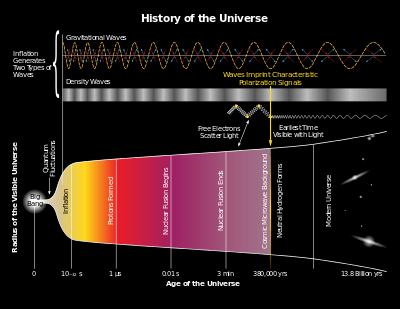
Gravitational waves should penetrate regions of space that electromagnetic waves cannot. It is hypothesized that they will be able to provide observers on Earth with information about black holes and other exotic objects in the distant Universe. Such systems cannot be observed with more traditional means such as optical telescopes or radio telescopes, and so gravitational-wave astronomy gives new insights into the working of the Universe. In particular, gravitational waves could be of interest to cosmologists as they offer a possible way of observing the very early Universe. This is not possible with conventional astronomy, since before recombination the Universe was opaque to electromagnetic radiation.[14] Precise measurements of gravitational waves will also allow scientists to test the general theory of relativity more thoroughly.
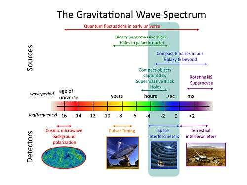
By studying gravitational waves, scientists will be able to discern what happened at the initial singularity.[15] In principle, gravitational waves could exist at any frequency. However, very low frequency waves would be impossible to detect and there is no credible source for detectable waves of very high frequency. Stephen Hawking and Werner Israel list different frequency bands for gravitational waves that could be plausibly detected, ranging from 10−7 Hz up to 1011 Hz.[16]
Effects of passing


The effects of a passing gravitational wave can be visualized by imagining a perfectly flat region of spacetime with a group of motionless test particles lying in a plane (e.g., the surface of a computer screen). As a gravitational wave passes through the particles along a line perpendicular to the plane of the particles (i.e. following the observer's line of vision into the screen), the particles will follow the distortion in spacetime, oscillating in a "cruciform" manner, as shown in the animations. The area enclosed by the test particles does not change and there is no motion along the direction of propagation.
The oscillations depicted in the animation are exaggerated for the purpose of discussion—in reality a gravitational wave has a very small amplitude (as formulated in linearized gravity). However, they help illustrate the kind of oscillations associated with gravitational waves as produced, for example, by a pair of masses in a circular orbit. In this case the amplitude of the gravitational wave is constant, but its plane of polarization changes or rotates at twice the orbital rate and so the time-varying gravitational wave size (or 'periodic spacetime strain') exhibits a variation as shown in the animation.[17] If the orbit is elliptical then the gravitational wave's amplitude also varies with time according to Einstein's quadrupole formula.[18]
As with other waves, there are a number of characteristics used to describe a gravitational wave:
- Amplitude: Usually denoted h, this is the size of the wave — the fraction of stretching or squeezing in the animation. The amplitude shown here is roughly h = 0.5 (or 50%). Gravitational waves passing through the Earth are many sextillion times weaker than this — h ≈ 10−20.
- Frequency: Usually denoted f, this is the frequency with which the wave oscillates (1 divided by the amount of time between two successive maximum stretches or squeezes)
- Wavelength: Usually denoted λ, this is the distance along the wave between points of maximum stretch or squeeze.
- Speed: This is the speed at which a point on the wave (for example, a point of maximum stretch or squeeze) travels. For gravitational waves with small amplitudes, this is equal to the speed of light (c).
The speed, wavelength, and frequency of a gravitational wave are related by the equation c = λ f, just like the equation for a light wave. For example, the animations shown here oscillate roughly once every two seconds. This would correspond to a frequency of 0.5 Hz, and a wavelength of about 600 000 km, or 47 times the diameter of the Earth.
In the above example, it is assumed that the wave is linearly polarized with a "plus" polarization, written h+. Polarization of a gravitational wave is just like polarization of a light wave except that the polarizations of a gravitational wave are at 45 degrees, as opposed to 90 degrees. In particular, in a "cross"-polarized gravitational wave, h×, the effect on the test particles would be basically the same, but rotated by 45 degrees, as shown in the second animation. Just as with light polarization, the polarizations of gravitational waves may also be expressed in terms of circularly polarized waves. Gravitational waves are polarized because of the nature of their sources.
Sources
In general terms, gravitational waves are radiated by objects whose motion involves acceleration, provided that the motion is not perfectly spherically symmetric (like an expanding or contracting sphere) or cylindrically symmetric (like a spinning disk or sphere). A simple example of this principle is a spinning dumbbell. If the dumbbell spins like a wheel on an axle, it will not radiate gravitational waves; if it tumbles end over end, as in the case of two planets orbiting each other, it will radiate gravitational waves. The heavier the dumbbell, and the faster it tumbles, the greater is the gravitational radiation it will give off. In an extreme case, such as when the two weights of the dumbbell are massive stars like neutron stars or black holes, orbiting each other quickly, then significant amounts of gravitational radiation would be given off.
Some more detailed examples:
- Two objects orbiting each other in a quasi-Keplerian planar orbit (basically, as a planet would orbit the Sun) will radiate.
- A spinning non-axisymmetric planetoid — say with a large bump or dimple on the equator — will radiate.
- A supernova will radiate except in the unlikely event that the explosion is perfectly symmetric.
- An isolated non-spinning solid object moving at a constant velocity will not radiate. This can be regarded as a consequence of the principle of conservation of linear momentum.
- A spinning disk will not radiate. This can be regarded as a consequence of the principle of conservation of angular momentum. However, it will show gravitomagnetic effects.
- A spherically pulsating spherical star (non-zero monopole moment or mass, but zero quadrupole moment) will not radiate, in agreement with Birkhoff's theorem.
More technically, the third time derivative of the quadrupole moment (or the l-th time derivative of the l-th multipole moment) of an isolated system's stress–energy tensor must be nonzero in order for it to emit gravitational radiation. This is analogous to the changing dipole moment of charge or current necessary for electromagnetic radiation.
Power radiated by orbiting bodies

Gravitational waves carry energy away from their sources and, in the case of orbiting bodies, this is associated with an inspiral or decrease in orbit. Imagine for example a simple system of two masses — such as the Earth–Sun system — moving slowly compared to the speed of light in circular orbits. Assume that these two masses orbit each other in a circular orbit in the x–y plane. To a good approximation, the masses follow simple Keplerian orbits. However, such an orbit represents a changing quadrupole moment. That is, the system will give off gravitational waves.
Suppose that the two masses are  and
and  , and they are separated by a distance
  . The power given off (radiated) by this system is:
 ,[19]
,[19]
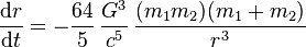
where G is the gravitational constant, c is the speed of light in vacuum and where the negative sign means that power is being given off by the system, rather than received. For a system like the Sun and Earth, is about 1.5×10¹¹ m and and are about 2×1030 and 6×1024 kg respectively. In this case, the power is about 200 watts. This is truly tiny compared to the total electromagnetic radiation given off by the Sun (roughly 3.86×1026 watts).
In theory, the loss of energy through gravitational radiation could eventually drop the Earth into the Sun. However, the total energy of the Earth orbiting the Sun (kinetic energy + gravitational potential energy) is about 1.14×1036 joules of which only 200 joules per second is lost through gravitational radiation, leading to a decay in the orbit by about 1×10⁻¹⁵ meters per day or roughly the diameter of a proton. At this rate, it would take the Earth approximately 1×10¹³ times more than the current age of the Universe to spiral onto the Sun. This estimate overlooks the decrease in r over time, but the majority of the time the bodies are far apart and only radiating slowly, so the difference is unimportant in this example.
A more dramatic example of radiated gravitational energy is represented by two solar mass (M☉) neutron stars orbiting at a distance from each other of 1.89×10⁸ m (only 0.63 light-seconds apart). [The Sun is 8 light minutes from the Earth.] Plugging their masses into the above equation shows that the gravitational radiation from them would be 1.38×1028 watts, which is about 100 times more than the Sun's electromagnetic radiation.
Orbital decay from gravitational radiation
Gravitational radiation robs the orbiting bodies of energy. It first circularizes their orbits and then gradually shrinks their radius. As the energy of the orbit is reduced, the distance between the bodies decreases, and they rotate more rapidly. The overall angular momentum is reduced however. This reduction corresponds to the angular momentum carried off by gravitational radiation. The rate of decrease of distance between the bodies versus time is given by:[19]
 ,
,
where the variables are the same as in the previous equation.
The orbit decays at a rate proportional to the inverse third power of the radius. When the radius has shrunk to half its initial value, it is shrinking eight times faster than before. By Kepler's Third Law, the new rotation rate at this point will be faster by  , or nearly three times the previous orbital frequency. As the radius decreases, the power lost to gravitational radiation increases even more. As can be seen from the previous equation, power radiated varies as the inverse fifth power of the radius, or 32 times more in this case.
Using the previous values for the Sun and the Earth, suggests that the Earth's orbit shrinks by 1.1×10⁻²⁰ meter per second. This is 3.5×10⁻¹³ m per year, which is about 1/300 the diameter of a hydrogen atom. The effect of gravitational radiation on the size of the Earth's orbit is unnoticeable over the age of the universe. Аctually, this effect is absolutely negligible compared to the increase of Earth's orbit due to losing mass of Sun via radiation (4.7×10⁻⁹ m/s).[20] This is not true for closer orbits.
A more practical example is the orbit of a Sun-like star around a heavy black hole. Our Milky Way is believed to have a 4 million M☉ black hole at its center in Sagittarius A. Such supermassive black holes are being found in the center of almost all galaxies. For this example take a 2 million M☉ black hole with a solar-mass star orbiting it at a radius of 1.89×10¹⁰ m (63 light-seconds). The mass of the black hole will be 4×1036 kg and its gravitational radius will be 6×10⁹ m. The orbital period will be 1,000 seconds, or a little under 17 minutes. The solar-mass star will draw closer to the black hole by 7.4 meters per second or 7.4 km per orbit. A collision will not be long in coming.
Assume that a pair of 1 M☉ neutron stars are in circular orbits at a distance of 1.89×10⁸ m (189,000 km). This is a little less than 1/7 the diameter of the Sun or 0.63 light-seconds. Their orbital period would be 1,000 seconds. Substituting the new mass and radius in the above formula gives a rate of orbit decrease of 3.7×10⁻⁶ m/s or 3.7 mm per orbit. This is 116 meters per year and is not negligible over cosmic time scales.
Suppose instead that these two neutron stars were orbiting at a distance of 1.89×10⁶ m (1890 km). Their period would be 1 second and their orbital velocity would be about 1/50 of the speed of light. Their orbit would now shrink by 3.7 meters per orbit. A collision is imminent. A runaway loss of energy from the orbit results in an ever more rapid decrease in the distance between the stars. They will eventually merge to form a black hole and cease to radiate gravitational waves. This is referred to as the inspiral.
The above equation can not be applied directly for calculating the lifetime of the orbit, because the rate of change in radius depends on the radius itself, and is thus non-constant with time. The lifetime can be computed by integration of this equation (see next section).
Orbital lifetime limits from gravitational radiation
Orbital lifetime is one of the most important properties of gravitational radiation sources. It determines the average number of binary stars in the universe that are close enough to be detected. Short lifetime binaries are strong sources of gravitational radiation but are few in number. Long lifetime binaries are more plentiful but they are weak sources of gravitational waves. LIGO is most sensitive in the frequency band where two neutron stars are about to merge. This time frame is only a few seconds. It takes luck for the detector to see this blink in time out of a million year orbital lifetime. It is predicted that such a merger will only be seen once per decade or so.
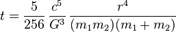
The lifetime of an orbit is given by:[19]
 ,
,
where r is the initial distance between the orbiting bodies. This equation can be derived by integrating the previous equation for the rate of radius decrease. It predicts the time for the radius of the orbit to shrink to zero. As the orbital speed becomes a significant fraction of the speed of light, this equation becomes inaccurate. It is useful for inspirals until the last few milliseconds before the merger of the objects.
Substituting the values for the mass of the Sun and Earth as well as the orbital radius gives a very large lifetime of 3.44×1030 seconds or 1.09×10²³ years (that is approximately 1013 times larger than the age of the universe). The actual figure would be slightly less than that. The Earth would break apart from tidal forces if it orbits closer than a few radii from the Sun. This would form a ring around the Sun, and the emission of gravitational waves would stop once the mass is distributed symmetrically around the Sun.
If computing a 2 million M☉ black hole with a solar mass star orbiting it at 1.89×10¹⁰ meters, it results on a lifetime of 6.50×10⁸ seconds or 20.7 years.
Assuming that a pair of solar mass neutron stars with a diameter of 10 kilometers are in circular orbits at a distance of 1.89×10⁸ m (189,000 km), and that their lifetime is 1.30×10¹³ seconds or about 414,000 years, then their orbital period would be 1,000 seconds and it could be observed by LISA if they were not too far away. A far greater number of white dwarf binaries exist with orbital periods in this range. White dwarf binaries have masses on the order of the Sun and diameters on the order of the Earth. They cannot get much closer together than 10,000 km before they will merge and explode in a supernova which will also end emission of gravitational waves. Until then, their gravitational radiation will be comparable to that of a neutron star binary.
If the orbit of a neutron star binary has decayed to 1.89×10⁶ m (1890 km), its remaining lifetime is 130,000 seconds or about 36 hours. The orbital frequency will vary from 1 revolution per second at the start and 918 revolutions per second when the orbit has shrunk to 20 km at merger. The gravitational radiation emitted will be at twice the orbital frequency. Just before merger, the inspiral can be observed by LIGO if the binary is close enough. LIGO has only a few minutes to observe this merger out of a total orbital lifetime that may have been billions of years. The chance of success with LIGO as initially constructed is quite low despite the large number of such mergers occurring in the universe, because the sensitivity of the instrument does not 'reach' out to enough systems to see events frequently. No mergers were seen in the few years that initial LIGO was in operation, and it is thought that a merger should be seen about once per several tens of years of observation time with initial LIGO.[21] The upgraded Advanced LIGO detector, with a ten times greater sensitivity, 'reaches' out 10 times further—encompassing a volume 1000 times greater, and seeing 1000 times as many candidate sources. Thus, the expectation is that detections will be made at the rate of tens per year.[22]
Wave amplitudes from the Earth–Sun system
We can also think in terms of the amplitude of the wave from a system in circular orbits. Let θ be the angle between the perpendicular to the plane of the orbit and the line of sight of the observer. Suppose that an observer is outside the system at a distance R from its center of mass. If R is much greater than a wavelength, the two polarizations of the wave will be
![h_{+} = -\frac{1}{R}\, \frac{G^2}{c^4}\, \frac{2 m_1 m_2}{r} (1+\cos^2\theta) \cos\left[2\omega(t - R/c)\right],](../I/m/57516c27a902dd502d0dae896ef5d856.png)
![h_{\times} = -\frac{1}{R}\, \frac{G^2}{c^4}\, \frac{4 m_1 m_2}{r}\, (\cos{\theta})\sin \left[2\omega(t-R/c)\right].](../I/m/c82de69587413e4f93a9b9453aa94ea9.png)
Here, we use the constant angular velocity of a circular orbit in Newtonian physics:

For example, if the observer is in the x-y plane then  , and
, and  , so the
  polarization is always zero. We also see that the frequency of the wave given off is twice the rotation frequency. If we put in numbers for the Earth–Sun system, we find:
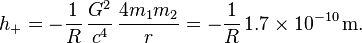
In this case, the minimum distance to find waves is R ≈ 1/4π light-year, so typical amplitudes will be h ≈ 10−25. That is, a ring of particles would stretch or squeeze by just one part in 1025. This is well under the detectability limit of all conceivable detectors.
Radiation from other sources
Although the waves from the Earth–Sun system are minuscule, astronomers can point to other sources for which the radiation should be substantial. One important example is the Hulse–Taylor binary — a pair of stars, one of which is a pulsar.[23] The characteristics of their orbit can be deduced from the Doppler shifting of radio signals given off by the pulsar. Each of the stars are about 1.4 M☉ and the size of their orbit is about 1/75 of the Earth–Sun orbit. This means the distance between the two stars is just a few times larger than the diameter of our own Sun. The combination of greater masses and smaller separation means that the energy given off by the Hulse–Taylor binary will be far greater than the energy given off by the Earth–Sun system — roughly 1022 times as much.
The information about the orbit can be used to predict just how much energy (and angular momentum) should be given off in the form of gravitational waves. As the energy is carried off, the stars should draw closer to each other. This effect is called an inspiral, and it can be observed in the pulsar's signals. The measurements on the Hulse–Taylor system have been carried out over more than 30 years. It has been shown that the gravitational radiation predicted by general relativity allows these observations to be matched within 0.2 percent. In 1993, Russell Hulse and Joe Taylor were awarded the Nobel Prize in Physics for this work, which was the first indirect evidence for gravitational waves. The orbital lifetime of this binary system before merger is a few hundred million years.[24]
Inspirals are very important sources of gravitational waves. Any time two compact objects (white dwarfs, neutron stars, or black holes) are in close orbits, they send out intense gravitational waves. As they spiral closer to each other, these waves become more intense. At some point they should become so intense that direct detection by their effect on objects on Earth or in space is possible. This direct detection is the goal of several large scale experiments.[25]
The only difficulty is that most systems like the Hulse–Taylor binary are so far away. The amplitude of waves given off by the Hulse–Taylor binary as seen on Earth would be roughly h ≈ 10−26. There are some sources, however, that astrophysicists expect to find with much larger amplitudes of h ≈ 10−20. At least eight other binary pulsars have been discovered.[26]
Astrophysics

During the past century, astronomy has been revolutionized by the use of new methods for observing the universe. Astronomical observations were originally made using visible light. Galileo Galilei pioneered the use of telescopes to enhance these observations. However, visible light is only a small portion of the electromagnetic spectrum, and not all objects in the distant universe shine strongly in this particular band. More useful information may be found, for example, in radio wavelengths. Using radio telescopes, astronomers have found pulsars, quasars, and other extreme objects that push the limits of our understanding of physics. Observations in the microwave band have opened our eyes to the faint imprints of the Big Bang, a discovery Stephen Hawking called the "greatest discovery of the century, if not all time". Similar advances in observations using gamma rays, x-rays, ultraviolet light, and infrared light have also brought new insights to astronomy. As each of these regions of the spectrum has opened, new discoveries have been made that could not have been made otherwise. Astronomers hope that the same holds true of gravitational waves.[27]
Gravitational waves have two important and unique properties. First, there is no need for any type of matter to be present nearby in order for the waves to be generated by a binary system of uncharged black holes, which would emit no electromagnetic radiation. Second, gravitational waves can pass through any intervening matter without being scattered significantly. Whereas light from distant stars may be blocked out by interstellar dust, for example, gravitational waves will pass through essentially unimpeded. These two features allow gravitational waves to carry information about astronomical phenomena never before observed by humans.
The sources of gravitational waves described above are in the low-frequency end of the gravitational-wave spectrum (10−7 to 105 Hz). An astrophysical source at the high-frequency end of the gravitational-wave spectrum (above 105 Hz and probably 1010 Hz) generates relic gravitational waves that are theorized to be faint imprints of the Big Bang like the cosmic microwave background (see gravitational wave background).[28] At these high frequencies it is potentially possible that the sources may be "man made"[16] that is, gravitational waves generated and detected in the laboratory.[29][30]
Energy, momentum, and angular momentum carried by gravitational waves
Water waves, sound waves, and electromagnetic waves are able to carry energy, momentum, and angular momentum. By carrying these away from a source, waves are able to rob that source of its energy as well as its linear and angular momentum. Gravitational waves perform the same function. Thus, for example, a binary system loses angular momentum as the two orbiting objects spiral towards each other—the angular momentum is radiated away by gravitational waves.
The waves can also carry off linear momentum, a possibility that has some interesting implications for astrophysics.[31] After two supermassive black holes coalesce, emission of linear momentum can produce a "kick" with amplitude as large as 4000 km/s. This is fast enough to eject the coalesced black hole completely from its host galaxy. Even if the kick is too small to eject the black hole completely, it can remove it temporarily from the nucleus of the galaxy, after which it will oscillate about the center, eventually coming to rest.[32] A kicked black hole can also carry a star cluster with it, forming a hyper-compact stellar system.[33] Or it may carry gas, allowing the recoiling black hole to appear temporarily as a "naked quasar". The quasar SDSS J092712.65+294344.0 is thought to contain a recoiling supermassive black hole.[34]
Detection

History
- 1915 – Albert Einstein publishes the theory of general relativity.
- 1916 – Albert Einstein predicts gravitational waves exist as a consequence of the theory of general relativity.[38][39]
- 1957 – Richard Feynman and Hermann Bondi predict if gravitational waves exist they are theoretically detectable by proposed sticky bead argument.[40]
- 1962 – M.E.Gertsenshtein and V.I.Pustovoit publish the first paper describing the principles to use interferometers to detect very long wavelength gravitational waves[41]
- 1968 – Joseph Weber reports gravitational waves have been detected, but the report findings prove to be false. Rainer Weiss analyzes Weber's method and starts conceiving LIGO[40]
- late 1970s – Indirect confirmation of the existence of gravitational waves, observations of a pair of pulsars show they move into tighter and faster orbits with an acceleration expected if they are losing energy by emitting gravitational waves.[42]
- 1984 – Kip Thorne, Ronald Drever and Rainier Weiss establish LIGO[40]
- 2002 – LIGO begins the search for gravitational waves[43]
- 17 March 2014 – Astronomers at the Harvard–Smithsonian Center for Astrophysics erroneously claim that they have detected and produce "the first direct image of gravitational waves" in the cosmic microwave background.[9][10][11][12][35][44]
- 2016 – A study by astrophysicists at Penn State University proposes that dark energy may distort gravitational waves, and cites this circumstance as a reason for a lack of direct detection.[45]
- 11 February 2016 – The Advanced LIGO team announce that they detected gravitational waves on 14 September 2015 from a merger of two black holes about 400 megaparsecs (1.3 billion light years) from Earth.[6][7][8] The merger event is named GW150914.[46]
Difficulties
Gravitational waves are not easily detectable. When they reach the Earth, they have a small amplitude with strain approximates 10−21, meaning that an extremely sensitive detector is needed, and that other sources of noise can overwhelm the signal.[47] Gravitational waves are expected to have frequencies 10−16 Hz < f < 104 Hz.[48]
Ground-based interferometers

Though the Hulse–Taylor observations were very important, they give only indirect evidence for gravitational waves. A more conclusive observation would be a direct measurement of the effect of a passing gravitational wave, which could also provide more information about the system that generated it. Any such direct detection is complicated by the extraordinarily small effect the waves would produce on a detector. The amplitude of a spherical wave will fall off as the inverse of the distance from the source (the 1/R term in the formulas for h above). Thus, even waves from extreme systems like merging binary black holes die out to very small amplitude by the time they reach the Earth. Astrophysicists expect that some gravitational waves passing the Earth may be as large as h ≈ 10−20, but generally no bigger.[49]
A simple device theorised to detect the expected wave motion is called a Weber bar — a large, solid bar of metal isolated from outside vibrations. This type of instrument was the first type of gravitational wave detector. Strains in space due to an incident gravitational wave excite the bar's resonant frequency and could thus be amplified to detectable levels. Conceivably, a nearby supernova might be strong enough to be seen without resonant amplification. With this instrument, Joseph Weber claimed to have detected daily signals of gravitational waves. His results, however, were contested in 1974 by physicists Richard Garwin and David Douglass. Modern forms of the Weber bar are still operated, cryogenically cooled, with superconducting quantum interference devices to detect vibration. Weber bars are not sensitive enough to detect anything but extremely powerful gravitational waves.[50]
MiniGRAIL is a spherical gravitational wave antenna using this principle. It is based at Leiden University, consisting of an exactingly machined 1150 kg sphere cryogenically cooled to 20 mK.[51] The spherical configuration allows for equal sensitivity in all directions, and is somewhat experimentally simpler than larger linear devices requiring high vacuum. Events are detected by measuring deformation of the detector sphere. MiniGRAIL is highly sensitive in the 2–4 kHz range, suitable for detecting gravitational waves from rotating neutron star instabilities or small black hole mergers.[52]

A more sensitive class of detector uses laser interferometry to measure gravitational-wave induced motion between separated 'free' masses.[53] This allows the masses to be separated by large distances (increasing the signal size); a further advantage is that it is sensitive to a wide range of frequencies (not just those near a resonance as is the case for Weber bars). Ground-based interferometers are now operational. Currently, the most sensitive is LIGO — the Laser Interferometer Gravitational Wave Observatory. LIGO has three detectors: one in Livingston, Louisiana, one at the Hanford site in Richland, Washington and a third (formerly installed as a second detector at Hanford) that is planned to be moved to India. Each observatory has two light storage arms that are 4 kilometers in length. These are at 90 degree angles to each other, with the light passing through 1 m diameter vacuum tubes running the entire 4 kilometers. A passing gravitational wave will slightly stretch one arm as it shortens the other. This is precisely the motion to which an interferometer is most sensitive.
Even with such long arms, the strongest gravitational waves will only change the distance between the ends of the arms by at most roughly 10−18 meters. LIGO should be able to detect gravitational waves as small as  . Upgrades to LIGO and other detectors such as Virgo, GEO 600, and TAMA 300 should increase the sensitivity still further; the next generation of instruments (Advanced LIGO and Advanced Virgo) will be more than ten times more sensitive. Another highly sensitive interferometer, KAGRA, is under construction in the Kamiokande mine in Japan. A key point is that a tenfold increase in sensitivity (radius of 'reach') increases the volume of space accessible to the instrument by one thousand times. This increases the rate at which detectable signals should be seen from one per tens of years of observation, to tens per year.[21]
Interferometric detectors are limited at high frequencies by shot noise, which occurs because the lasers produce photons randomly; one analogy is to rainfall—the rate of rainfall, like the laser intensity, is measurable, but the raindrops, like photons, fall at random times, causing fluctuations around the average value. This leads to noise at the output of the detector, much like radio static. In addition, for sufficiently high laser power, the random momentum transferred to the test masses by the laser photons shakes the mirrors, masking signals at low frequencies. Thermal noise (e.g., Brownian motion) is another limit to sensitivity. In addition to these 'stationary' (constant) noise sources, all ground-based detectors are also limited at low frequencies by seismic noise and other forms of environmental vibration, and other 'non-stationary' noise sources; creaks in mechanical structures, lightning or other large electrical disturbances, etc. may also create noise masking an event or may even imitate an event. All these must be taken into account and excluded by analysis before a detection may be considered a true gravitational wave event.
There are currently two detectors focused on the higher end of the gravitational wave spectrum (10−7 to 105 Hz): one at University of Birmingham, England,[54] and the other at INFN Genoa, Italy. A third is under development at Chongqing University, China. The Birmingham detector measures changes in the polarization state of a microwave beam circulating in a closed loop about one meter across. Both detectors are expected to be sensitive to periodic spacetime strains of  , given as an amplitude spectral density. The INFN Genoa detector is a resonant antenna consisting of two coupled spherical superconducting harmonic oscillators a few centimeters in diameter. The oscillators are designed to have (when uncoupled) almost equal resonant frequencies. The system is currently expected to have a sensitivity to periodic spacetime strains of
  , with an expectation to reach a sensitivity of
  . The Chongqing University detector is planned to detect relic high-frequency gravitational waves with the predicted typical parameters ~1011 Hz (100 GHz) and h ~10−30 to 10−32.[55]
Einstein@Home
The simplest gravitational waves are those with constant frequency. The waves given off by a spinning, non-axisymmetric neutron star would be approximately monochromatic: a pure tone in acoustics. Unlike signals from supernovae of binary black holes, these signals evolve little in amplitude or frequency over the period it would be observed by ground-based detectors. However, there would be some change in the measured signal, because of Doppler shifting caused by the motion of the Earth. Despite the signals being simple, detection is extremely computationally expensive, because of the long stretches of data that must be analysed.
The Einstein@Home project is a distributed computing project similar to SETI@home intended to detect this type of gravitational wave. By taking data from LIGO and GEO, and sending it out in little pieces to thousands of volunteers for parallel analysis on their home computers, Einstein@Home can sift through the data far more quickly than would be possible otherwise.[56]
Space-based interferometers
Space-based interferometers, such as LISA and DECIGO, are also being developed. LISA's design calls for three test masses forming an equilateral triangle, with lasers from each spacecraft to each other spacecraft forming two independent interferometers. LISA is planned to occupy a solar orbit trailing the Earth, with each arm of the triangle being five million kilometers. This puts the detector in an excellent vacuum far from Earth-based sources of noise, though it will still be susceptible to shot noise, as well as artifacts caused by cosmic rays and solar wind.
Using pulsar timing arrays
Pulsars are rapidly rotating stars. A pulsar emits beams of radio waves that, like lighthouse beams, sweep through the sky as the pulsar rotates. The signal from a pulsar can be detected by radio telescopes as a series of regularly spaced pulses, essentially like the ticks of a clock. Gravitational waves affect the time it takes the pulses to travel from the pulsar to a telescope on Earth. A pulsar timing array uses millisecond pulsars to seek out perturbations due to gravitational waves in measurements of pulse arrival times at a telescope, in other words, to look for deviations in the clock ticks. In particular, pulsar timing arrays can search for a distinct pattern of correlation and anti-correlation between the signals over an array of different pulsars (resulting in the name "pulsar timing array"). Although pulsar pulses travel through space for hundreds or thousands of years to reach us, pulsar timing arrays are sensitive to perturbations in their travel time of much less than a millionth of a second.
Globally there are three active pulsar timing array projects. The North American Nanohertz Gravitational Wave Observatory uses data collected by the Arecibo Radio Telescope and Green Bank Telescope. The Parkes Pulsar Timing Array at the Parkes radio-telescope has been collecting data since March 2005. The European Pulsar Timing Array uses data from the four largest telescopes in Europe: the Lovell Telescope, the Westerbork Synthesis Radio Telescope, the Effelsberg Telescope and the Nancay Radio Telescope. (Upon completion the Sardinia Radio Telescope will be added to the EPTA also.) These three projects have begun collaborating under the title of the International Pulsar Timing Array project.
Primordial
Primordial gravitational waves are gravitational waves observed in the cosmic microwave background. They were allegedly detected by the BICEP2 instrument, an announcement made on 17 March 2014, which was withdrawn on 30 January 2015 ("the signal can be entirely attributed to dust in the Milky Way"[37]).
LIGO gravitational wave observation, 2015
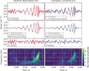
On 11 February 2016, the LIGO collaboration announced the detection of gravitational waves, from a signal detected at 10:51 GMT on 14 September 2015[57] of two black holes with masses of 29 and 36 solar masses merging together about 1.3 billion light years away. During the final fraction of a second of the collision, It released more power than 50 times of all the stars in the observable universe combined.[58] The signal sweeps upwards in frequency from 35 to 250 Hz.[7] The mass of the new black hole obtained from merging the two was 62 solar masses. Energy equivalent to three solar masses was emitted as gravitational waves.[59] The signal was seen by both LIGO detectors, in Livingston and Hanford, with a time difference of 7 milliseconds due to the angle between the two detectors and the source. The signal came from the Southern Celestial Hemisphere, in the rough direction of (but much further away than) the Magellanic Clouds.[6] The confidence level of this being an observation of gravitational waves was 99.99994%.[59]
Mathematics
Einstein's equations form the fundamental law of general relativity. The curvature of spacetime can be expressed mathematically using the metric tensor — denoted  . The metric holds information regarding how distances are measured in the space under consideration. Because the propagation of gravitational waves through space and time change distances, we will need to use this to find the solution to the wave equation.
Spacetime curvature is also expressed with respect to a covariant derivative,  , in the form of the Einstein tensor,
  . This curvature is related to the stress–energy tensor,
  , by the key equation
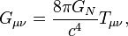
where  is Newton's gravitational constant, and
  is the speed of light. We assume geometrized units, so
  .
.
With some simple assumptions, Einstein's equations can be rewritten to show explicitly that they are wave equations. To begin with, we adopt some coordinate system, like  . We define the flat-space metric
  to be the quantity that — in this coordinate system — has the components we would expect for the flat space metric. For example, in these spherical coordinates, we have
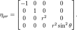
This flat-space metric has no physical significance; it is a purely mathematical device necessary for the analysis. Tensor indices are raised and lowered using this "flat-space metric".
Now, we can also think of the physical metric as a matrix, and find its determinant,  . Finally, we define a quantity

This is the crucial field, which will represent the radiation. It is possible (at least in an asymptotically flat spacetime) to choose the coordinates in such a way that this quantity satisfies the de Donder gauge condition (conditions on the coordinates):
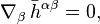
where represents the flat-space derivative operator. These equations say that the divergence of the field is zero. The linear Einstein equations can now be written[60] as
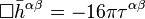 ,
,
where 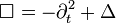 represents the flat-space d'Alembertian operator, and
  represents the stress–energy tensor plus quadratic terms involving
  . This is just a wave equation for the field with a source, despite the fact that the source involves terms quadratic in the field itself. That is, it can be shown that solutions to this equation are waves traveling with velocity 1 in these coordinates.
Linear approximation
The equations above are valid everywhere — near a black hole, for instance. However, because of the complicated source term, the solution is generally too difficult to find analytically. We can often assume that space is nearly flat, so the metric is nearly equal to the  tensor. In this case, we can neglect terms quadratic in , which means that the field reduces to the usual stress–energy tensor
  . That is, Einstein's equations become
 .
.
If we are interested in the field far from a source, however, we can treat the source as a point source; everywhere else, the stress–energy tensor would be zero, so
 .
.
Now, this is the usual homogeneous wave equation — one for each component of . Solutions to this equation are well known. For a wave moving away from a point source, the radiated part (meaning the part that dies off as  far from the source) can always be written in the form
  , where
  is just some function. It can be shown[61] that — to a linear approximation — it is always possible to make the field traceless. Now, if we further assume that the source is positioned at
  , the general solution to the wave equation in spherical coordinates is
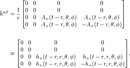
where we now see the origin of the two polarizations.
Relation to the source
If we know the details of a source — for instance, the parameters of the orbit of a binary — we can relate the source's motion to the gravitational radiation observed far away. With the relation
- ,
we can write the solution in terms of the tensorial Green's function for the d'Alembertian operator:[60]
 .
.
Though it is possible to expand the Green's function in tensor spherical harmonics, it is easier to simply use the form
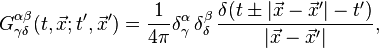
where the positive and negative signs correspond to ingoing and outgoing solutions, respectively. Generally, we are interested in the outgoing solutions, so
 .
.
If the source is confined to a small region very far away, to an excellent approximation we have:
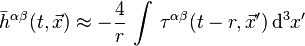 ,
,
where  .
.
Now, because we will eventually only be interested in the spatial components of this equation (time components can be set to zero with a coordinate transformation), and we are integrating this quantity — presumably over a region of which there is no boundary — we can put this in a different form. Ignoring divergences with the help of Stokes' theorem and an empty boundary, we can see that
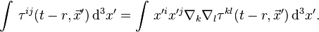
Inserting this into the above equation, we arrive at
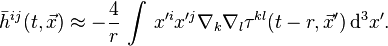
Finally, because we have chosen to work in coordinates for which  , we know that
  . With a few simple manipulations, we can use this to prove that
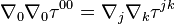 .
.
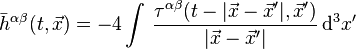
With this relation, the expression for the radiated field is
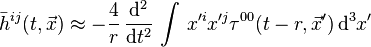 .
.
In the linear case,  , the density of mass-energy.
To a very good approximation, the density of a simple binary can be described by a pair of delta-functions, which eliminates the integral. Explicitly, if the masses of the two objects are  and
and  , and the positions are
  and
and  , then
 .
.
We can use this expression to do the integral above:
 .
.
Using mass-centered coordinates, and assuming a circular binary, this is
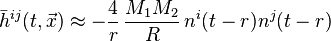 ,
,
where  . Plugging in the known values of
  , we obtain the expressions given above for the radiation from a simple binary.
In fiction
An episode of the Russian science-fiction novel Space Apprentice by Arkady and Boris Strugatsky shows the experiment monitoring the propagation of gravitational waves at the expense of annihilating a chunk of 15 Eunomia the size of Everest. The novel was written in 1961 and published in 1962, exactly at the time when Soviet physicists Michail Gerstenstein and Vladislav Pustovoit prepared and published their proposal on using laser interferometry for gravitational wave detection.[62]
See also
- First observation of gravitational waves
- Gravitational field
- Gravitational-wave astronomy
- Gravitational wave background
- Gravitational-wave observatory
- Gravitomagnetism
- Graviton (and Gravitational wave observation#Gravitons)
- Hawking radiation, for gravitationally induced electromagnetic radiation from black holes
- HM Cancri
- LISA, DECIGO and BBO — Proposed space-based detectors
- LIGO, Virgo interferometer, GEO600, KAGRA, and TAMA 300 — Ground-based gravitational-wave detectors
- Linearised Einstein field equations
- Peres metric
- pp-wave spacetime, for an important class of exact solutions modelling gravitational radiation
- PSR B1913+16, the first binary pulsar to be discovered and the first experimental evidence for the existence of gravitational waves.
- Spin-flip, a consequence of gravitational wave emission from binary supermassive black holes
- Sticky bead argument, for a physical way to see that gravitational radiation should carry energy
- Tidal force
References
- ↑ Einstein, A (June 1916). "Näherungsweise Integration der Feldgleichungen der Gravitation". Sitzungsberichte der Königlich Preussischen Akademie der Wissenschaften Berlin. part 1: 688–696.
- ↑ Einstein, A (1918). "Über Gravitationswellen". Sitzungsberichte der Königlich Preussischen Akademie der Wissenschaften Berlin. part 1: 154–167.
- ↑ Finley, Dave. "Einstein's gravity theory passes toughest test yet: Bizarre binary star system pushes study of relativity to new limits.". Phys.Org.
- ↑ The Detection of Gravitational Waves using LIGO, B. Barish
- ↑ "The Newest Search for Gravitational Waves has Begun". LIGO Caltech. LIGO. 18 September 2015. Retrieved 29 November 2015.
- 1 2 3 Castelvecchi, Davide; Witze, Witze (February 11, 2016). "Einstein's gravitational waves found at last". Nature News. doi:10.1038/nature.2016.19361. Retrieved 2016-02-11.
- 1 2 3 B. P. Abbott et al. (LIGO Scientific Collaboration and Virgo Collaboration) (2016). "Observation of Gravitational Waves from a Binary Black Hole Merger". Physical Review Letters 116 (6). doi:10.1103/PhysRevLett.116.061102.
- 1 2 "Gravitational waves detected 100 years after Einstein's prediction | NSF - National Science Foundation". www.nsf.gov. Retrieved 2016-02-11.
- 1 2 3 Staff (17 March 2014). "BICEP2 2014 Results Release". National Science Foundation. Retrieved 18 March 2014.
- 1 2 3 Clavin, Whitney (17 March 2014). "NASA Technology Views Birth of the Universe". NASA. Retrieved 17 March 2014.
- 1 2 3 Overbye, Dennis (17 March 2014). "Detection of Waves in Space Buttresses Landmark Theory of Big Bang". New York Times. Retrieved 17 March 2014.
- 1 2 "First Second of the Big Bang". How The Universe Works 3. 2014. Discovery Science.
- ↑ LIGO Scientific Collaboration; Virgo Collaboration (2012). "Search for Gravitational Waves from Low Mass Compact Binary Coalescence in LIGO's Sixth Science Run and Virgo's Science Runs 2 and 3". Physical Review D 85: 082002. arXiv:1111.7314. Bibcode:2012PhRvD..85h2002A. doi:10.1103/PhysRevD.85.082002.
- ↑ Krauss, LM; Dodelson, S; Meyer, S (2010). "Primordial Gravitational Waves and Cosmology". Science 328 (5981): 989–992. arXiv:1004.2504. Bibcode:2010Sci...328..989K. doi:10.1126/science.1179541. PMID 20489015.
- ↑ Radford, Tim (2016-02-11). "Gravitational waves: breakthrough discovery after two centuries of expectation". The Guardian. ISSN 0261-3077. Retrieved 2016-02-11.
- 1 2 Hawking, S. W.; Israel, W. (1979). General Relativity: An Einstein Centenary Survey. Cambridge: Cambridge University Press. p. 98. ISBN 0-521-22285-0.
- ↑ Landau, L. D.; Lifshitz, E. M. (1975). The Classical Theory of Fields (Fourth Revised English ed.). Pergamon Press. pp. 356–357. ISBN 0-08-025072-6.
- ↑ Einstein, A (1918). "Über Gravitationswellen". Sitzungsberichte, Preussische Akademie der Wissenschaften 154.
- 1 2 3 Gravitational Radiation
- ↑ Beatty, Kelly. "Why is the Earth moving away from the sun?". New Scientist.
- 1 2 LIGO Scientific Collaboration; Virgo Collaboration (2010). "Predictions for the rates of compact binary coalescences observable by ground-based gravitational-wave detectors". Classical and Quantum Gravity 27: 17300. arXiv:1003.2480. Bibcode:2010CQGra..27q3001A. doi:10.1088/0264-9381/27/17/173001.
- ↑ LIGO Scientific Collaboration - FAQ; section: "Do we expect LIGO's advanced detectors to make a discovery, then?" and "What's so different about LIGO's advanced detectors?", retrieved 14 February 2016
- ↑ Relativistic Binary Pulsar B1913+16: Thirty Years of Observations and Analysis
- ↑ "[1411.3930] 1974: the discovery of the first binary pulsar".
- ↑ Crashing Black Holes
- ↑ Binary and Millisecond Pulsars
- ↑ Berry, Christopher (14 May 2015). "Listening to the gravitational universe: what can’t we see?". University of Birmingham. University of Birmingham. Retrieved 29 November 2015.
- ↑ L. P. Grishchuk (1976), "Primordial Gravitons and the Possibility of Their Observation", Sov. Phys. JETP Lett. 23, p. 293.
- ↑ Braginsky, V. B., Rudenko and Valentin, N. Section 7: "Generation of gravitational waves in the laboratory", Physics Report (Review section of Physics Letters), 46, No. 5. 165–200, (1978).
- ↑ Li, Fangyu, Baker, R. M L, Jr., and Woods, R. C., "Piezoelectric-Crystal-Resonator High-Frequency Gravitational Wave Generation and Synchro-Resonance Detection", in the proceedings of Space Technology and Applications International Forum (STAIF-2006), edited by M.S. El-Genk, AIP Conference Proceedings, Melville NY 813: 2006.
- ↑ Merritt, D.; et al. (May 2004). "Consequences of Gravitational Wave Recoil". The Astrophysical Journal Letters 607 (1): L9–L12. arXiv:astro-ph/0402057. Bibcode:2004ApJ...607L...9M. doi:10.1086/421551.
- ↑ Gualandris, A.; Merritt, D.; et al. (May 2008). "Ejection of Supermassive Black Holes from Galaxy Cores". The Astrophysical Journal 678 (2): 780–797. arXiv:0708.0771. Bibcode:2008ApJ...678..780G. doi:10.1086/586877.
- ↑ Merritt, D.; Schnittman, J. D.; Komossa, S. (2009). "Hypercompact Stellar Systems Around Recoiling Supermassive Black Holes". The Astrophysical Journal 699 (2): 1690–1710. arXiv:0809.5046. Bibcode:2009ApJ...699.1690M. doi:10.1088/0004-637X/699/2/1690.
- ↑ Komossa, S.; Zhou, H.; Lu, H. (May 2008). "A Recoiling Supermassive Black Hole in the Quasar SDSS J092712.65+294344.0?". The Astrophysical Journal 678 (2): L81–L84. arXiv:0804.4585. Bibcode:2008ApJ...678L..81K. doi:10.1086/588656
- 1 2 "First Direct Evidence of Cosmic Inflation". www.cfa.harvard.edu. Harvard-Smithsonian Center for Astrophysics. 17 March 2014. Retrieved 17 March 2014.
- ↑ Overbye, Dennis (24 March 2014). "Ripples From the Big Bang". New York Times. Retrieved 24 March 2014.
- 1 2 Cowen, Ron (2015-01-30). "Gravitational waves discovery now officially dead". nature. doi:10.1038/nature.2015.16830.
- ↑ "The long road towards evidence". Alexander Blum, Roberto Lalli and Jürgen Renn. Max Planck Society. 2016-02-12. Retrieved 2016-02-14.
- ↑ "APS -81st Annual Meeting of the APS Southeastern Section - Event - Status of Advanced LIGO detectors". meetings.aps.org. Retrieved 2016-02-12.
- 1 2 3 "Gravitational Waves Discovered at Long Last | Quanta Magazine". www.quantamagazine.org. Retrieved 2016-02-12.
- ↑ Gertsenshtein, M. E.; Pustovoit, V. I. (August 1962). "On the detection of low frequency gravitational waves". JETP 43: 605–607.
- ↑ Paul McNamara (2016-02-11). "ESA CONGRATULATIONS ON GRAVITATIONAL WAVE DISCOVERY". ESA. Archived from the original on 2016-02-11. Retrieved 2016-02-12.
- ↑ "Facts". LIGO Lab | Caltech. Retrieved 2016-02-15.
- ↑ Ian Sample. "Gravitational waves turn to dust after claims of flawed analysis". the Guardian.
- ↑ "Dark Energy May Be Distorting Our View of Gravitational Waves". MotherBoard. 2016.
- ↑ "LIGO detects first ever gravitational waves – from two merging black holes - physicsworld.com". physicsworld.com. Retrieved 2016-02-12.
- ↑ "Noise and Sensitivity". gwoptics: Gravitational wave E-book. University of Birmingham. Retrieved 10 December 2015.
- ↑ Thorne, Kip S. (1995). "Gravitational Waves". arXiv:gr-qc/9506086.
- ↑ David G. Blair (Ed.) (1991). The detection of gravitational waves. Cambridge University Press.
- ↑ For a review of early experiments using Weber bars, see Levine, J. (April 2004). "Early Gravity-Wave Detection Experiments, 1960–1975". Physics in Perspective (Birkhäuser Basel) 6 (1): 42–75. Bibcode:2004PhP.....6...42L. doi:10.1007/s00016-003-0179-6.
- ↑ "MiniGRAIL, the first spherical gravitational wave detector".
- ↑ de Waard, Arlette; Luciano Gottardi; Giorgio Frossati (July 2000). Spherical Gravitational Wave Detectors: cooling and quality factor of a small CuAl6% sphere (PDF). Marcel Grossmann meeting on General Relativity. Rome, Italy: World Scientific Publishing Co. Pte. Ltd. (published December 2002). pp. 1899–1901. Bibcode:2002nmgm.meet.1899D. doi:10.1142/9789812777386_0420. ISBN 9789812777386.
- ↑ The idea of using laser interferometry for gravitational wave detection was first mentioned by Gerstenstein and Pustovoit 1963 Sov. Phys.–JETP 16 433. Weber mentioned it in an unpublished laboratory notebook. Rainer Weiss first described in detail a practical solution with an analysis of realistic limitations to the technique in R. Weiss (1972). "Electromagetically Coupled Broadband Gravitational Antenna". Quarterly Progress Report, Research Laboratory of Electronics, MIT 105: 54.
- ↑ Cruise, Mike. "Research Interests". Astrophysics & Space Research Group. University of Birmingham. Retrieved 29 November 2015.
- ↑ High Frequency Relic Gravitational Waves. page 12
- ↑ "Einstein@Home".
- ↑ "Gravitational waves from black holes detected". BBC News. 11 February 2016.
- ↑ This collision was 50 times more powerful than all the stars in the universe combined
- 1 2 LIGO’s First-Ever Detection of Gravitational Waves Opens a New Window on the Universe
- 1 2 Thorne, Kip (April 1980). "Multipole expansions of gravitational radiation". Reviews of Modern Physics 52 (2): 299–339. Bibcode:1980RvMP...52..299T. doi:10.1103/RevModPhys.52.299.
- ↑ C. W. Misner, K. S. Thorne, and J. A. Wheeler (1973). Gravitation. W. H. Freeman and Co.
- ↑ ME Gerstenstein, VI Pustovoit (1962). "On the Detection of Low-Frequency Gravitational Waves". ZhETF (in Russian) 16 (8): 605–607. Bibcode:1963JETP...16..433G.
Further reading
- Bartusiak, Marcia. Einstein's Unfinished Symphony. Washington, DC: Joseph Henry Press, 2000.
- Chakrabarty, Indrajit, "Gravitational Waves: An Introduction". arXiv:physics/9908041 v1, Aug 21, 1999.
- Landau, L. D. and Lifshitz, E. M., The Classical Theory of Fields (Pergamon Press), 1987..
- Will, Clifford M., The Confrontation between General Relativity and Experiment. Living Reviews Relativity 9 (2006) 3.
- Peter Saulson, Fundamentals of Interferometric Gravitational Wave Detectors, World Scientific, 1994.
Bibliography
- Berry, Michael, Principles of Сosmology and Gravitation (Adam Hilger, Philadelphia, 1989). ISBN 0-85274-037-9
- Collins, Harry, Gravity's Shadow: The Search for Gravitational Waves, University of Chicago Press, 2004.
- P. J. E. Peebles, Principles of Physical Cosmology (Princeton University Press, Princeton, 1993). ISBN 0-691-01933-9.
- Wheeler, John Archibald and Ciufolini, Ignazio, Gravitation and Inertia (Princeton University Press, Princeton, 1995). ISBN 0-691-03323-4.
- Woolf, Harry, ed., Some Strangeness in the Proportion (Addison–Wesley, Reading, Massachusetts, 1980). ISBN 0-201-09924-1.
External links
| Wikimedia Commons has media related to Gravitational waves. |
| Look up gravitational wave in Wiktionary, the free dictionary. |
- Gravitational waves at Encyclopædia Britannica
- Laser Interferometer Gravitational Wave Observatory. LIGO Laboratory, operated by the California Institute of Technology and the Massachusetts Institute of Technology
- Caltech Relativity Tutorial – A basic introduction to gravitational waves
- Video (04:36) – Detecting a gravitational wave, Dennis Overbye, NYT (11 February 2016).
- Video (71:29) – Press Conference announcing discovery: "LIGO detects gravitational waves", National Science Foundation (11 February 2016).
| ||||||||||||||||||||||||||||||||||||||

| ||||||||||||||||||||||||||||||||||||||||||||||||||||||||
|