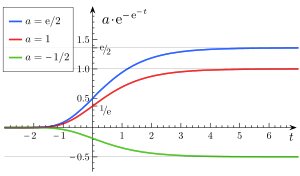
Gompertz function

A Gompertz curve or Gompertz function, named after Benjamin Gompertz, is a sigmoid function. It is a type of mathematical model for a time series, where growth is slowest at the start and end of a time period. The right-hand or future value asymptote of the function is approached much more gradually by the curve than the left-hand or lower valued asymptote, in contrast to the simple logistic function in which both asymptotes are approached by the curve symmetrically. It is a special case of the generalised logistic function.

**Graphs of Gompertz curves, showing the effect of varying one of a,b,c while keeping the others constant**
Varying $a$
Varying $b$
Varying $c$

Formula

y(t)=ae^{-be^{-ct}}

where

a is an asymptote, since $ae^{be^{- \infty }}=ae^0=a$
b, c are positive numbers
b sets the displacement along the x axis (translates the graph to the left or right)
c sets the growth rate (y scaling)
e is Euler's Number (e = 2.71828...)

Derivation

The function curve can be derived from a Gompertz law of mortality, which states the rate of mortality (decay) falls exponentially with current size. Mathematically

k^{r} \propto \frac{1}{y(t)}

where

$r=\frac{y'(t)}{y(t)}$ is the rate of growth.
k is an arbitrary constant.

Example uses

Examples of uses for Gompertz curves include:

Mobile phone uptake, where costs were initially high (so uptake was slow), followed by a period of rapid growth, followed by a slowing of uptake as saturation was reached.^[1]
Population in a confined space, as birth rates first increase and then slow as resource limits are reached.^[2]

Modeling of growth of tumors
Modelling market impact in finance.^[3]

Growth of tumors

In the 1960s A.K. Laird^[4] for the first time successfully used the Gompertz curve to fit data of growth of tumors. In fact, tumors are cellular populations growing in a confined space where the availability of nutrients is limited. Denoting the tumor size as X(t) it is useful to write the Gompertz Curve as follows:

X(t) = K \exp\left( \log\left( \frac{X(0)}{K} \right) \exp\left(-\alpha t \right) \right)

where:

X(0) is the tumor size at the starting observation time;
K is the carrying capacity, i.e. the maximum size that can be reached with the available nutrients. In fact it is:

\lim_{t \rightarrow +\infty}X(t)=K

independently on X(0)>0. Note that, in absence of therapies etc.. usually it is X(0)<K, whereas, in presence of therapies, it may be X(0)>K;

α is a constant related to the proliferative ability of the cells.
log() refers to the natural log.

It is easy to verify that the dynamics of X(t) is governed by the Gompertz differential equation:

X^{\prime}(t) = \alpha \log\left( \frac{K}{X(t)} \right) X(t)

i.e. is of the form:

X^{\prime}(t) = F\left( X(t) \right) X(t), F^{\prime}(X) \le 0

where F(X) is the instantaneous proliferation rate of the cellular population, whose decreasing nature is due to the competition for the nutrients due to the increase of the cellular population, similarly to the logistic growth rate. However, there is a fundamental difference: in the logistic case the proliferation rate for small cellular population is finite:

F(X) = \alpha \left( 1 - \left(\frac{X}{K}\right)^{\nu}\right) \Rightarrow F(0)=\alpha < +\infty

whereas in the Gompertz case the proliferation rate is unbounded:

\lim_{X \rightarrow 0^{+} } F(X) = \lim_{X \rightarrow 0^{+} } \alpha \log\left( \frac{K}{X}\right) = +\infty

As noticed by Steel^[5] and by Wheldon,^[6] the proliferation rate of the cellular population is ultimately bounded by the cell division time. Thus, this might be an evidence that the Gompertz equation is not good to model the growth of small tumors. Moreover, more recently it has been noticed^[7] that, including the interaction with immune system, Gompertz and other laws characterized by unbounded F(0) would preclude the possibility of immune surveillance.

Gompertz growth and logistic growth

The Gompertz differential equation

X^{\prime}(t) = \alpha \log\left( \frac{K}{X(t)} \right) X(t)

is the limiting case of the generalized logistic differential equation

X^{\prime}(t) = \alpha \nu \left( 1 - \left(\frac{X(t)}{K}\right)^{\frac{1}{\nu}} \right) X(t)

(where $\nu > 0$ is a positive real number) since

\lim_{\nu \rightarrow +\infty} \nu \left( 1 - x^{1/\nu} \right) = -\log \left( x \right)

In addition, there is an inflection point in the graph of the generalized logistic function when

X(t) = \left( \frac{\nu}{\nu+1} \right)^{\nu} K

and one in the graph of the Gompertz function when

X(t) = \frac{K}{e} = K \cdot \lim_{\nu \rightarrow +\infty} \left( \frac{\nu}{\nu+1} \right)^{\nu}

Gomp-ex law of growth

Based on the above considerations, Wheldon^[6] proposed a mathematical model of tumor growth, called the Gomp-Ex model, that slightly modifies the Gompertz law. In the Gomp-Ex model it is assumed that initially there is no competition for resources, so that the cellular population expands following the exponential law. However, there is a critical size threshold $X_{C}$ such that for $X>X_{C}$ the growth follows the Gompertz Law:

F(X)=\max\left(a,\alpha \log\left( \frac{K}{X}\right) \right)

so that:

X_{C}= K \exp\left(-\frac{a}{\alpha}\right).

Here there are some numerical estimates^[6] for $X_{C}$ :

$X_{C}\approx 10^9$ for human tumors
$X_{C}\approx 10^6$ for murine (mouse) tumors

References

↑ Islam, Towhidul; Fiebig, Denzil G.; Meade, Nigel (2002), "Modelling multinational telecommunications demand with limited data", International Journal of Forecasting 18 (4): 605–624, doi:10.1016/S0169-2070(02)00073-0 .
↑ Zwietering, M. H.; Jongenburger, I.; Rombout, F. M.; van 't Riet, K. (1990), "Modeling of the Bacterial Growth Curve", Applied and Environmental Microbiology 56 (6): 1875–1881 .
↑ Caravelli, F.; Sindoni, L.; Caccioli, F.; Ududec, C. (2015), Optimal leverage trajectories in presence of market impact .
↑ Laird A. K. (1964). "Dynamics of tumor growth". Br J of Cancer 18 (3): 490–502. doi:10.1038/bjc.1964.55.
↑ Steel, G.G. (1977). Growth Kinetics of Tumors. Oxford: Clarendon Press. ISBN 0-19-857388-X.
1 2 3 Wheldon, T.E. (1988). Mathematical Models in Cancer Research. Bristol: Adam Hilger. ISBN 0-85274-291-6.
↑ d'Onofrio A. (2005). "A general framework for modeling tumor-immune system competition and immunotherapy: Mathematical analysis and biomedical inferences". Physica D 208 (3–4): 220–235. doi:10.1016/j.physd.2005.06.032.

External links

Weisstein, Eric W., "Gompertz Curve", MathWorld.

This article is issued from Wikipedia - version of the Saturday, October 31, 2015. The text is available under the Creative Commons Attribution/Share Alike but additional terms may apply for the media files.