General matrix notation of a VAR(p)

This page shows the details for different matrix notations of a vector autoregression process with k variables.

Var(p)

y_t =c + A_1 y_{t-1} + A_2 y_{t-2} + \cdots + A_p y_{t-p} + e_t, \,

Where each $y_{i}$ is a vector of length k and each $A_i$ is a k × k matrix.

Large matrix notation

\begin{bmatrix}y_{1,t} \\ y_{2,t}\\ \vdots \\ y_{k,t}\end{bmatrix}=\begin{bmatrix}c_{1} \\ c_{2}\\ \vdots \\ c_{k}\end{bmatrix}+ \begin{bmatrix} a_{1,1}^1&a_{1,2}^1 & \cdots & a_{1,k}^1\\ a_{2,1}^1&a_{2,2}^1 & \cdots & a_{2,k}^1\\ \vdots& \vdots& \ddots& \vdots\\ a_{k,1}^1&a_{k,2}^1 & \cdots & a_{k,k}^1 \end{bmatrix} \begin{bmatrix}y_{1,t-1} \\ y_{2,t-1}\\ \vdots \\ y_{k,t-1}\end{bmatrix} + \cdots + \begin{bmatrix} a_{1,1}^p&a_{1,2}^p & \cdots & a_{1,k}^p\\ a_{2,1}^p&a_{2,2}^p & \cdots & a_{2,k}^p\\ \vdots& \vdots& \ddots& \vdots\\ a_{k,1}^p&a_{k,2}^p & \cdots & a_{k,k}^p \end{bmatrix} \begin{bmatrix}y_{1,t-p} \\ y_{2,t-p}\\ \vdots \\ y_{k,t-p}\end{bmatrix} + \begin{bmatrix}e_{1,t} \\ e_{2,t}\\ \vdots \\ e_{k,t}\end{bmatrix}

Equation by regression notation

Rewriting the y variables one to one gives:

$y_{1,t} = c_{1} + a_{1,1}^1y_{1,t-1} + a_{1,2}^1y_{2,t-1} +\cdots + a_{1,k}^1y_{k,t-1}+\cdots+a_{1,1}^py_{1,t-p}+a_{1,2}^py_{2,t-p}+ \cdots +a_{1,k}^py_{k,t-p} + e_{1,t}\,$

$y_{2,t} = c_{2} + a_{2,1}^1y_{1,t-1} + a_{2,2}^1y_{2,t-1} +\cdots + a_{2,k}^1y_{k,t-1}+\cdots+a_{2,1}^py_{1,t-p}+a_{2,2}^py_{2,t-p}+ \cdots +a_{2,k}^py_{k,t-p} + e_{2,t}\,$

$\qquad\vdots$

$y_{k,t} = c_{k} + a_{k,1}^1y_{1,t-1} + a_{k,2}^1y_{2,t-1} +\cdots + a_{k,k}^1y_{k,t-1}+\cdots+a_{k,1}^py_{1,t-p}+a_{k,2}^py_{2,t-p}+ \cdots +a_{k,k}^py_{k,t-p} + e_{k,t}\,$

Concise matrix notation

One can rewrite a VAR(p) with k variables in a general way which includes T+1 observations $y_0$ through $y_T$

Y=BZ +U \,

Where:

Y= \begin{bmatrix}y_{p} & y_{p+1} & \cdots & y_{T}\end{bmatrix} = \begin{bmatrix}y_{1,p} & y_{1,p+1} & \cdots & y_{1,T} \\ y_{2,p} &y_{2,p+1} & \cdots & y_{2,T}\\ \vdots& \vdots &\vdots &\vdots \\ y_{k,p} &y_{k,p+1} & \cdots & y_{k,T}\end{bmatrix}

B= \begin{bmatrix} c & A_{1} & A_{2} & \cdots & A_{p} \end{bmatrix} = \begin{bmatrix} c_{1} & a_{1,1}^1&a_{1,2}^1 & \cdots & a_{1,k}^1 &\cdots & a_{1,1}^p&a_{1,2}^p & \cdots & a_{1,k}^p\\ c_{2} & a_{2,1}^1&a_{2,2}^1 & \cdots & a_{2,k}^1 &\cdots & a_{2,1}^p&a_{2,2}^p & \cdots & a_{2,k}^p \\ \vdots & \vdots& \vdots& \ddots& \vdots & \cdots & \vdots& \vdots& \ddots& \vdots\\ c_{k} & a_{k,1}^1&a_{k,2}^1 & \cdots & a_{k,k}^1 &\cdots & a_{k,1}^p&a_{k,2}^p & \cdots & a_{k,k}^p \end{bmatrix}

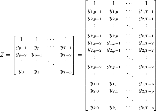
Z= \begin{bmatrix} 1 & 1 & \cdots & 1 \\ y_{p-1} & y_{p} & \cdots & y_{T-1}\\ y_{p-2} & y_{p-1} & \cdots & y_{T-2}\\ \vdots & \vdots & \ddots & \vdots\\ y_{0} & y_{1} & \cdots & y_{T-p} \end{bmatrix} = \begin{bmatrix} 1 & 1 & \cdots & 1 \\ y_{1,p-1} & y_{1,p} & \cdots & y_{1,T-1} \\ y_{2,p-1} & y_{2,p} & \cdots & y_{2,T-1} \\ \vdots & \vdots & \ddots & \vdots\\ y_{k,p-1} & y_{k,p} & \cdots & y_{k,T-1} \\ y_{1,p-2} & y_{1,p-1} & \cdots & y_{1,T-2} \\ y_{2,p-2} & y_{2,p-1} & \cdots & y_{2,T-2} \\ \vdots & \vdots & \ddots & \vdots\\ y_{k,p-2} & y_{k,p-1} & \cdots & y_{k,T-2} \\ \vdots & \vdots & \ddots & \vdots\\ y_{1,0} & y_{1,1} & \cdots & y_{1,T-p} \\ y_{2,0} & y_{2,1} & \cdots & y_{2,T-p} \\ \vdots & \vdots & \ddots & \vdots\\ y_{k,0} & y_{k,1} & \cdots & y_{k,T-p} \end{bmatrix}

and

U= \begin{bmatrix} e_{p} & e_{p+1} & \cdots & e_{T} \end{bmatrix}= \begin{bmatrix} e_{1,p} & e_{1,p+1} & \cdots & e_{1,T} \\ e_{2,p} & e_{2,p+1} & \cdots & e_{2,T} \\ \vdots & \vdots & \ddots & \vdots \\ e_{k,p} & e_{k,p+1} & \cdots & e_{k,T} \end{bmatrix}.

One can then solve for the coefficient matrix B (e.g. using an ordinary least squares estimation of $Y \approx BZ$ )

References

Lütkepohl, Helmut (2005). New Introduction to Multiple Time Series Analysis. Berlin: Springer. ISBN 3540401725.

This article is issued from Wikipedia - version of the Monday, January 19, 2015. The text is available under the Creative Commons Attribution/Share Alike but additional terms may apply for the media files.