Fei–Ranis model of economic growth
| Economics |
|---|
_Per_Capita_in_2014.svg.png) |
|
|
| By application |
|
| Lists |
|
The Fei–Ranis model of economic growth is a dualism model in developmental economics or welfare economics that has been developed by John C. H. Fei and Gustav Ranis and can be understood as an extension of the Lewis model. It is also known as the Surplus Labor model. It recognizes the presence of a dual economy comprising both the modern and the primitive sector and takes the economic situation of unemployment and underemployment of resources into account, unlike many other growth models that consider underdeveloped countries to be homogenous in nature.[1] According to this theory, the primitive sector consists of the existing agricultural sector in the economy, and the modern sector is the rapidly emerging but small industrial sector.[2] Both the sectors co-exist in the economy, wherein lies the crux of the development problem. Development can be brought about only by a complete shift in the focal point of progress from the agricultural to the industrial economy, such that there is augmentation of industrial output. This is done by transfer of labor from the agricultural sector to the industrial one, showing that underdeveloped countries do not suffer from constraints of labor supply. At the same time, growth in the agricultural sector must not be negligible and its output should be sufficient to support the whole economy with food and raw materials. Like in the Harrod–Domar model, saving and investment become the driving forces when it comes to economic development of underdeveloped countries.[1]
Basics of the model
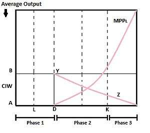
One of the biggest drawbacks of the Lewis model was the undermining of the role of agriculture in boosting the growth of the industrial sector. In addition to that, he did not acknowledge that the increase in productivity of labor should take place prior to the labor shift between the two sectors. However, these two ideas were taken into account in the Fei–Ranis dual economy model of three growth stages.[3] They further argue that the model lacks in the proper application of concentrated analysis to the change that takes place with agricultural development[4] In Phase 1 of the Fei–Ranis model, the elasticity of the agricultural labor work-force is infinite and as a result, suffers from disguised unemployment. Also, the marginal product of labor is zero. This phase is similar to the Lewis model.In Phase 2 of the model, the agricultural sector sees a rise in productivity and this leads to increased industrial growth such that a base for the next phase is prepared. In Phase 2, agricultural surplus may exist as the increasing average product (AP), higher than the marginal product (MP) and not equal to the subsistence level of wages.[5]
Using the help of the figure on the left, we see that
According to Fei and Ranis, AD amount of labor (see figure) can be shifted from the agricultural sector without any fall in output. Hence, it represents surplus labor.

After AD, MP begins to rise, and industrial labor rises from zero to a value equal to AD. AP of agricultural labor is shown by BYZ and we see that this curve falls downward after AD. This fall in AP can be attributed to the fact that as agricultural laborers shift to the industrial sector, the real wage of industrial laborers decreases due to shortage of food supply, since less laborers are now working in the food sector. The decrease in the real wage level decreases the level of profits, and the size of surplus that could have been re-invested for more industrialization. However, as long as surplus exists, growth rate can still be increased without a fall in the rate of industrialization. This re-investment of surplus can be graphically visualized as the shifting of MP curve outwards. In Phase2 the level of disguised unemployment is given by AK.[3] This allows the agricultural sector to give up a part of its labor-force until
Phase 3 begins from the point of commercialization which is at K in the Figure. This is the point where the economy becomes completely commercialized in the absence of disguised unemployment. The supply curve of labor in Phase 3 is steeper and both the sectors start bidding equally for labor.
The amount of labor that is shifted and the time that this shifting takes depends upon:
- The growth of surplus generated within the agricultural sector, and the growth of industrial capital stock dependent on the growth of industrial profits;
- The nature of the industry's technical progress and its associated bias;
- Growth rate of population.[3]
So, the three fundamental ideas used in this model are:
- Agricultural growth and industrial growth are both equally important;
- Agricultural growth and industrial growth are balanced;
- Only if the rate at which labor is shifted from the agricultural to the industrial sector is greater than the rate of growth of population will the economy be able to lift itself up from the Malthusian population trap.[3]
This shifting of labor can take place by the landlords' investment activities and by the government's fiscal measures. However, the cost of shifting labor in terms of both private and social cost may be high, for example transportation cost or the cost of carrying out construction of buildings. In addition to that, per capita agricultural consumption can increase, or there can exist a wide gap between the wages of the urban and the rural people. These three occurrences- high cost, high consumption and high gap in wages, are called as leakages, and leakages prevent the creation of agricultural surplus. In fact, surplus generation might be prevented due to a backward-sloping supply curve of labor as well, which happens when high income-levels are not consumed. This would mean that the productivity of laborers with rise in income will not rise. However, the case of backward-sloping curves is mostly unpractical.[3]
Connectivity between sectors
Fei and Ranis emphasized strongly on the industry-agriculture interdependency and said that a robust connectivity between the two would encourage and speedup development. If agricultural laborers look for industrial employment, and industrialists employ more workers by use of larger capital good stock and labor-intensive technology, this connectivity can work between the industrial and agricultural sector. Also, if the surplus owner invests in that section of industrial sector that is close to soil and is in known surroundings, he will most probably choose that productivity out of which future savings can be channelized. They took the example of Japan's dualistic economy in the 19th century and said that connectivity between the two sectors of Japan was heightened due the presence of a decentralized rural industry which was often linked to urban production. According to them, economic progress is achieved in dualistic economies of underdeveloped countries through the work of a small number of entrepreneurs who have access to land and decision-making powers and use industrial capital and consumer goods for agricultural practices.
Agricultural sector
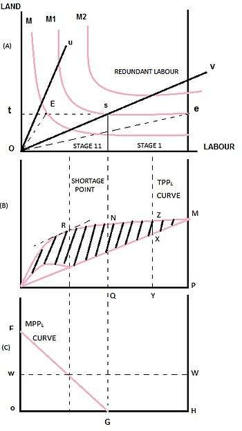
In (A), land is measured on the vertical axis, and labor on the horizontal axis. Ou and Ov represent two ridge lines, and the production contour lines are depicted by M, M1 and M2. The area enclosed by the ridge lines defines the region of factor substitutability, or the region where factors can easily be substituted. Let us understand the repercussions of this. If te amount of labor is the total labor in the agricultural sector, the intersection of the ridge line Ov with the production curve M1 at point s renders M1 perfectly horizontal below Ov. The horizontal behavior of the production line implies that outside the region of factor substitutability, output stops and labor becomes redundant once land is fixed and labor is increased.[6]
If Ot is the total land in the agricultural sector, ts amount of labor can be employed without it becoming redundant, and es represents the redundant agricultural labor force. This led Fei and Ranis to develop the concept of Labor Utilization Ratio, which they define as the units of labor that can be productively employed (without redundancy) per unit of land. In the left-side figure, labor utilization ratio
which is graphically equal to the inverted slope of the ridge line Ov.
Fei and Ranis also built the concept of endowment ratio, which is a measure of the relative availability of the two factors of production. In the figure, if Ot represents agricultural land and tE represents agricultural labor, then the endowment ratio is given by
which is equal to the inverted slope of OE. The actual point of endowment is given by E.
Finally, Fei and Ranis developed the concept of non-redundancy coefficient T which is measured by
These three concepts helped them in formulating a relationship between T, R and S. If :: then
then
This mathematical relation proves that the non-redundancy coefficient is directly proportional to labor utilization ratio and is inversely proportional to the endowment ratio.
(B) displays the total physical productivity of labor (TPPL) curve. The curve increases at a decreasing rate, as more units of labor are added to a fixed amount of land. At point N, the curve shapes horizontally and this point N conforms to the point G in (C, which shows the marginal productivity of labor (MPPL) curve, and with point s on the ridge line Ov in (A).
Industrial sector
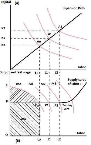
Like in the agricultural sector, Fei and Ranis assume constant returns to scale in the industrial sector. However, the main factors of production are capital and labor. In the graph (A) right hand side, the production functions have been plotted taking labor on the horizontal axis and capital on the vertical axis. The expansion path of the industrial sector is given by the line OAoA1A2. As capital increases from Ko to K1 to K2 and labor increases from Lo to L1 and L2, the industrial output represented by the production contour Ao, A1 and A3 increases accordingly.
According to this model, the prime labor supply source of the industrial sector is the agricultural sector, due to redundancy in the agricultural labor force. (B) shows the labor supply curve for the industrial sector S. PP2 represents the straight line part of the curve and is a measure of the redundant agricultural labor force on a graph with industrial labor force on the horizontal axis and output/real wage on the vertical axis. Due to the redundant agricultural labor force, the real wages remain constant but once the curve starts sloping upwards from point P2, the upward sloping indicates that additional labor would be supplied only with a corresponding rise in the real wages level.
MPPL curves corresponding to their respective capital and labor levels have been drawn as Mo, M1, M2 and M3. When capital stock rises from Ko to K1, the marginal physical productivity of labor rises from Mo to M1. When capital stock is Ko, the MPPL curve cuts the labor supply curve at equilibrium point Po. At this point, the total real wage income is Wo and is represented by the shaded area POLoPo. λ is the equilibrium profit and is represented by the shaded area qPPo. Since the laborers have extremely low income-levels, they barely save from that income and hence industrial profits (πo) become the prime source of investment funds in the industrial sector.
Here, Kt gives the total supply of investment funds (given that rural savings are represented by So)
Total industrial activity rises due to increase in the total supply of investment funds, leading to increased industrial employment.
Agricultural surplus
Agricultural surplus in general terms can be understood as the produce from agriculture which exceeds the needs of the society for which it is being produced, and may be exported or stored for future use.
Generation of agricultural surplus
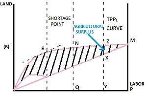
To understand the formation of agricultural surplus,we must refer to graph (B) of the agricultural sector. The figure on the left is a reproduced version of a section of the previous graph, with certain additions to better explain the concept of agricultural surplus. We first derive the average physical productivity of the total agricultural labor force (APPL). Fei and Ranis hypothesize that it is equal to the real wage and this hypothesis is known as the constant institutional wage hypothesis. It is also equal in value to the ratio of total agricultural output to the total agricultural population. Using this relation, we can obtain APPL = MP/OP. This is graphically equal to the slope of line OM, and is represented by the line WW in (C).
Observe point Y, somewhere to the left of P on the graph. If a section of the redundant agricultural labor force (PQ) is removed from the total agricultural labor force (OP) and absorbed into the industrial sector, then the labor force remaining in the industrial sector is represented by the point Y. Now, the output produced by the remaining labor force is represented by YZ and the real income of this labor force is given by XY. The difference of the two terms yields the total agricultural surplus of the economy. It is important to understand that this surplus is produced by the reallocation of labor such that it is absorbed by the industrial sector. This can be seen as deployment of hidden rural savings for the expansion of the industrial sector. Hence, we can understand the contribution of the agricultural sector to the expansion of industrial sector by this allocation of redundant labor force and the agricultural surplus that results from it.
Agricultural surplus as wage fund

Agricultural surplus plays a major role as a wage fund. Its importance can be better explained with the help of the graph on the right, which is an integration of the industrial sector graph with an inverted agricultural sector graph, such that the origin of the agricultural sector falls on the upper-right corner. This inversion of the origin changes the way the graph is now perceived. While the labor force values are read from the left of 0, the output values are read vertically downwards from O. The sole reason for this inversion is for the sake of convenience. The point of commercialization as explained before (See Section on Basics of the model) is observed at point R, where the tangent to the line ORX runs parallel to OX.
Before a section of the redundant labor force is absorbed into the industrial sector, the entire labor OA is present in the agricultural sector. Once AG amount of labor force (say) is absorbed, it represented by OG' in the industrial sector, and the labor remaining in the agricultural sector is then OG. But how is the quantity of labor absorbed into the industrial sector determined? (A) shows the supply curve of labor SS' and several demand curves for labor df, d'f' and d"f". When the demand for labor is df, the intersection of the demand-supply curves gives the equilibrium employment point G'. Hence OG represents the amount of labor absorbed into the industrial sector. In that case, the labor remaining in the agricultural sector is OG. This OG amount of labor produces an output of GF, out of which GJ amount of labor is consumed by the agricultural sector and JF is the agricultural surplus for that level of employment. Simultaneously, the unproductive labor force from the agricultural sector turns productive once it is absorbed by the industrial sector, and produces an output of OG'Pd as shown in the graph, earning a total wage income of OG'PS.
The agricultural surplus JF created is needed for consumption by the same workers who left for the industrial sector. Hence, agriculture successfully provides not only the manpower for production activities elsewhere, but also the wage fund required for the process.
Significance of agriculture in the Fei–Ranis model
The Lewis model is criticised on the grounds that it neglects agriculture. Fei–Ranis model goes a step beyond and states that agriculture has a very major role to play in the expansion of the industrial sector. In fact, it says that the rate of growth of the industrial sector depends on the amount of total agricultural surplus and on the amount of profits that are earned in the industrial sector. So, larger the amount of surplus and the amount of surplus put into productive investment and larger the amount of industrial profits earned, the larger will be the rate of growth of the industrial economy. As the model focuses on the shifting of the focal point of progress from the agricultural to the industrial sector, Fei and Ranis believe that the ideal shifting takes place when the investment funds from surplus and industrial profits are sufficiently large so as to purchase industrial capital goods like plants and machinery. These capital goods are needed for the creation of employment opportunities. Hence, the condition put by Fei and Ranis for a successful transformation is that
Rate of increase of capital stock & rate of employment opportunities > Rate of population growth
The indispensability of labor reallocation
As an underdeveloped country goes through its development process, labor is reallocated from the agricultural to the industrial sector. More the rate of reallocation, faster is the growth of that economy. The economic rationale behind this idea of labor reallocation is that of faster economic development. The essence of labor reallocation lies in Engel's Law, which states that the proportion of income being spent on food decreases with increase in the income-level of an individual, even if there is a rise in the actual expenditure on food. For example, if 90 per cent of the entire population of the concerned economy is involved in agriculture, that leaves just 10 per cent of the population in the industrial sector. As the productivity of agriculture increases, it becomes possible for just 35 per cent of population to maintain a satisfactory food supply for the rest of the population. As a result, the industrial sector now has 65 per cent of the population under it. This is extremely desirable for the economy, as the growth of industrial goods is subject to the rate of per capita income, while the growth of agricultural goods is subject only to the rate of population growth, and so a bigger labor supply to the industrial sector would be welcome under the given conditions. In fact, this labor reallocation becomes necessary with time since consumers begin to want more of industrial goods than agricultural goods in relative terms.
However, Fei and Ranis were quick to mention that the necessity of labor reallocation must be linked more to the need to produce more capital investment goods as opposed to the thought of industrial consumer goods following the discourse of Engel's Law. This is because the assumption that the demand for industrial goods is high seems unrealistic, since the real wage in the agricultural sector is extremely low and that hinders the demand for industrial goods. In addition to that, low and mostly constant wage rates will render the wage rates in the industrial sector low and constant. This implies that demand for industrial goods will not rise at a rate as suggested by the use of Engel's Law.
Since the growth process will observes a slow-paced increase in the consumer purchasing power, the dualistic economies follow the path of natural austerity, which is characterized by more demand and hence importance of capital good industries as compared to consumer good ones. However, investment in capital goods comes with a long gestation period, which drives the private entrepreneurs away. This suggests that in order to enable growth, the government must step in and play a major role, especially in the initial few stages of growth. Additionally, the government also works on the social and economic overheads by the construction of roads, railways, bridges, educational institutions, health care facilities and so on.
Growth without development
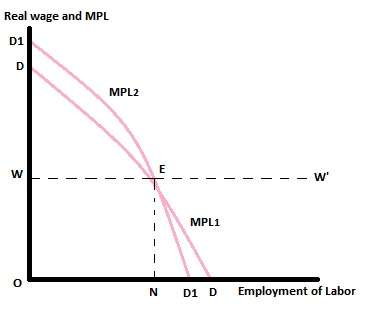
In the Fei-Ranis model, it is possible that as technological progress takes place and there is a shift to labor-saving production techniques, growth of the economy takes place with increase in profits but no economic development takes place. This can be explained well with the help of graph in this section.
The graph displays two MPL lines plotted with real wage and MPL on the vertical axis and employment of labor on the horizontal axis. OW denotes the subsistence wage level, which is the minimum wage level at which a worker (and his family) would survive. The line WW' running parallel to the X-axis is considered to be infinitely elastics since supply of labor is assumed to be unlimited at the subsistence-wage level. The square area OWEN represents the wage bill and DWE represents the surplus or the profits collected. This surplus or profit can increase if the MPL curve changes.[3]
If the MPL curve changes from MPL1 to MPL2 due to a change in production technique, such that it becomes labor-saving or capital-intensive, then the surplus or profit collected would increase. This increase can be seen by comparing DWE with D1WE since D1WE since is greater in area compared to DWE. However, there is no new point of equilibrium and as E continues to be the point of equilibrium,there is no increase in the level of labor employment, or in wages for that matter. Hence, labor employment continues as ON and wages as OW. The only change that accompanies the change in production technique is the one in surplus or profits.[3]
This makes for a good example of a process of growth without development, since growth takes place with increase in profits but development is at a standstill since employment and wages of laborers remain the same.
[3]
Reactions to the model

Fei–Ranis model of economic growth has been criticized on multiple grounds, although if the model is accepted, then it will have a significant theoretical and policy implications on the underdeveloped countries' efforts towards development and on the persisting controversial statements regarding the balanced vs. unbalanced growth debate.[7]
- It has been asserted that Fei and Ranis did not have a clear understanding of the sluggish economic situation prevailing in the developing countries. If they had thoroughly scrutinized the existing nature and causes of it, they would have found that the existing agricultural backwardness was due to the institutional structure, primarily the system of feudalism that prevailed.[8]
- Fei and Ranis say, "It has been argued that money is not a simple substitute for physical capital in an aggregate production function. There are reasons to believe that the relationship between money and physical capital could be complementary to one another at some stage of economic development, to the extent that credit policies could play an important part in easing bottlenecks on the growth of agriculture and industry." This indicates that in the process of development they neglect the role of money and prices. They fail to differ between wage labor and household labor, which is a significant distinction for evaluating prices of dualistic development in an underdeveloped economy.[8]
- Fei and Ranis assume that MPPL is zero during the early phases of economic development, which has been criticized by Harry T.Oshima and some others on the grounds that MPPL of labor is zero only if the agricultural population is very large, and if it is very large, some of that labor will shift to cities in search of jobs. In the short run, this section of labor that has shifted to the cities remains unemployed, but over the long run it is either absorbed by the informal sector, or it returns to the villages and attempts to bring more marginal land into cultivation. They have also neglected seasonal unemployment, which occurs due to seasonal change in labor demand and is not permanent.[8]
To understand this better, we refer to the graph in this section, which shows Food on the vertical axis and Leisure on the horizontal axis. OS represents the subsistence level of food consumption, or the minimum level of food consumed by agricultural labor that is necessary for their survival. I0 and I1 between the two commodities of food and leisure (of the agriculturists). The origin falls on G, such that OG represents maximum labor and labor input would be measured from the right to the left. The transformation curve SAG falls from A, which indicates that more leisure is being used to same units of land. At A, the marginal transformation between food and leisure and MPL = 0 and the indifference curve I0 is also tangent to the transformation curve at this point. This is the point of leisure satiation.
Consider a case where a laborer shifts from the agricultural to the industrial sector. In that case, the land left behind would be divided between the remaining laborers and as a result, the transformation curve would shift from SAG to RTG. Like at point A, MPL at point T would be 0 and APL would continue to be the same as that at A (assuming constant returns to scale). If we consider MPL = 0 as the point where agriculturalists live on the subsistence level, then the curve RTG must be flat at point T in order to maintain the same level of output. However, that would imply leisure satiation or leisure as an inferior good, which are two extreme cases. It can be surmised then that under normal cases, the output would decline with shift of labor to industrial sector, although the per capita output would remain the same. This is because, a fall in the per capita output would mean fall in consumption in a way that it would be lesser than the subsistence level, and the level of labor input per head would either rise or fall.
Berry and Soligo in their 1968 paper have criticized this model for its MPL=0 assumption, and for the assumption that the transfer of labor from the agricultural sector leaves the output in that sector unchanged in Phase 1. They show that the output changes, and may fall under various land tenure systems, unless the following situations arise:[3]
1. Leisure falls under the inferior good category 2. Leisure satiation is present. 3. There is perfect substitutability between food and leisure, and the marginal rate of substitution is constant for all real income levels.
Now if MPL>0 then leisure satiation option becomes invalid, and if MPL=0 then the option of food and leisure as perfect substitutes becomes invalid. Therefore, the only remaining viable option is leisure as an inferior good.
- While mentioning the important role of high agricultural productivity and the creation of surplus for economic development, they have failed to mention the need for capital as well. Although it is important to create surplus, it is equally important to maintain it through technical progress, which is possible through capital accumulation, but the Fei-Ranis model considers only labor and output as factors of production.[3]
- The question of whether MPL = 0 is that of an empirical one. The underdeveloped countries mostly exhibit seasonality in food production, which suggests that especially during favorable climatic conditions, say that of harvesting or sowing, MPL would definitely be greater than zero.[3]
- Fei and Ranis assume a close model and hence there is no presence of foreign trade in the economy, which is very unrealistic as food or raw materials can not be imported. If we take the example of Japan again, the country imported cheap farm products from other countries and this made better the country's terms of trade.[8] Later they relaxed the assumption and said that the presence of a foreign sector was allowed as long as it was a "facilitator" and not the main driving force.[7]
- The reluctant expansionary growth in the industrial sector of underdeveloped countries can be attributed to the lagging growth in the productivity of subsistence agriculture. This suggests that increase in surplus becomes more important a determinant as compared to re-investment of surplus, an idea that was utilized by Jorgenson in his 1961 model that centered around the necessity of surplus generation and surplus persistence.[3]
- Stagnation has not been taken into consideration, and no distinction is made between labor through family and labor through wages. There is also no explanation of the process of self-sustained growth, or of the investment function. There is complete negligence of terms of trade between agriculture and industry, foreign exchange, money and price.[3]
References
- 1 2 "Economnics4Development Website". Surplus Labor Model of Economic Development. Retrieved 12 October 2011.
- ↑ Thirlwall, A.P (2006). Growth and Development: With Special Reference to Developing Economies. Palgrave Macmillan. ISBN 1-4039-9600-8.
- 1 2 3 4 5 6 7 8 9 10 11 12 13 Subrata, Ghatak (2003). Introduction to Developmental Economics. London: Routledge. ISBN 0-415-09722-3.
- ↑ "Ranis-Fei model vs. Lewis Model" (PDF). Developmentafrique.com. Retrieved 14 October 2011.
- ↑ "American Economic Review". The Ranis-Fei Model of Economic Development: Comment 53: 448–452. JSTOR 1809172.
- ↑ Ranis, Gustav. "Paper on Labor Surplus Economies" (PDF). Retrieved 4 October 2011.
- 1 2 J. Choo, Hakchung. "American Economic Review". On the Empirical Relevancy of the Rans-Fei Model of Economic Development: Comment 61: 695–703. JSTOR 1811863.
- 1 2 3 4 Misra, Puri, S.K, V.K (2010). Economics of Development and Planning. Mumbai, India: Himalaya Publishing House. pp. 270–279. ISBN 978-81-8488-829-4.
| ||||||


