Euler–Lagrange equation

In calculus of variations, the Euler–Lagrange equation, Euler's equation,^[1] or Lagrange's equation (although the latter name is ambiguous—see disambiguation page), is a second-order partial differential equation whose solutions are the functions for which a given functional is stationary. It was developed by Swiss-Russian mathematician Leonhard Euler and French-Italian mathematician Joseph-Louis Lagrange in the 1750s.

Because a differentiable functional is stationary at its local maxima and minima, the Euler–Lagrange equation is useful for solving optimization problems in which, given some functional, one seeks the function minimizing (or maximizing) it. This is analogous to Fermat's theorem in calculus, stating that at any point where a differentiable function attains a local extremum, its derivative is zero.

In Lagrangian mechanics, because of Hamilton's principle of stationary action, the evolution of a physical system is described by the solutions to the Euler–Lagrange equation for the action of the system. In classical mechanics, it is equivalent to Newton's laws of motion, but it has the advantage that it takes the same form in any system of generalized coordinates, and it is better suited to generalizations. In classical field theory there is an analogous equation to calculate the dynamics of a field.

History

The Euler–Lagrange equation was developed in the 1750s by Euler and Lagrange in connection with their studies of the tautochrone problem. This is the problem of determining a curve on which a weighted particle will fall to a fixed point in a fixed amount of time, independent of the starting point.

Lagrange solved this problem in 1755 and sent the solution to Euler. Both further developed Lagrange's method and applied it to mechanics, which led to the formulation of Lagrangian mechanics. Their correspondence ultimately led to the calculus of variations, a term coined by Euler himself in 1766.^[2]

Statement

The Euler–Lagrange equation is an equation satisfied by a function, q, of a real argument, t, which is a stationary point of the functional

\displaystyle S(\boldsymbol q) = \int_a^b L(t,\boldsymbol q(t),\boldsymbol q'(t))\, \mathrm{d}t

where:

$\boldsymbol q$ is the function to be found:

\begin{align} \boldsymbol q \colon [a, b] \subset \mathbb{R} & \to X \\ t & \mapsto x = \boldsymbol q(t) \end{align}

such that

\boldsymbol q

is differentiable,

\boldsymbol q(a) = \boldsymbol x_a

, and

\boldsymbol q(b) = \boldsymbol x_{b}

;

$\boldsymbol q'$ ; is the derivative of $\boldsymbol q$ :
$\begin{align} q' \colon [a, b] & \to T_{q(t)}X \\ t & \mapsto v = q'(t) \end{align}$

TX being the tangent bundle of X defined by

TX = \bigcup_{x \in X} \{ x \} \times T_{x}X

;

L is a real-valued function with continuous first partial derivatives:
$\begin{align} L \colon [a, b] \times TX & \to \mathbb{R} \\ (t, x, v) & \mapsto L(t, x, v). \end{align}$

The Euler–Lagrange equation, then, is given by

$L_x(t,q(t),q'(t))-\frac{\mathrm{d}}{\mathrm{d}t}L_v(t,q(t),q'(t)) = 0.$

where L_x and L_v denote the partial derivatives of L with respect to the second and third arguments, respectively.

If the dimension of the space X is greater than 1, this is a system of differential equations, one for each component:

\frac{\partial L}{\partial q_i}(t,\boldsymbol q(t),\boldsymbol q'(t))-\frac{\mathrm{d}}{\mathrm{d}t}\frac{\partial L}{\partial \dot q_i}(t,\boldsymbol q(t),\boldsymbol q'(t)) = 0 \quad \text{for } i = 1, \dots, n.

Derivation of one-dimensional Euler–Lagrange equation

The derivation of the one-dimensional Euler–Lagrange equation is one of the classic proofs in mathematics. It relies on the fundamental lemma of calculus of variations.

We wish to find a function $f$ which satisfies the boundary conditions $f(a) = A$ , $f(b) = B$ , and which extremizes the functional

J = \int_a^b F(x,f(x),f'(x))\, \mathrm{d}x\ . \,\!

We assume that $F$ is twice continuously differentiable.^[3] A weaker assumption can be used, but the proof becomes more difficult.

If $f$ extremizes the functional subject to the boundary conditions, then any slight perturbation of $f$ that preserves the boundary values must either increase $J$ (if $f$ is a minimizer) or decrease $J$ (if $f$ is a maximizer).

Let $g_{\varepsilon} (x) = f (x) + \varepsilon \eta (x)$ be the result of such a perturbation $\varepsilon \eta (x)$ of $f$ , where $\varepsilon$ is small and $\eta (x)$ is a differentiable function satisfying $\eta (a) = \eta (b) = 0$ . Then define

J_\varepsilon = \int_a^b F(x,g_\varepsilon(x), g_\varepsilon'(x) ) \, \mathrm{d}x = \int_a^b F_\varepsilon\, \mathrm{d}x \,\!

where $F_\varepsilon = F(x, \, g_\varepsilon (x), \, g_\varepsilon' (x) )$ .

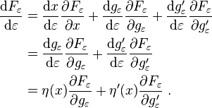
We now wish to calculate the total derivative of $J_\varepsilon$ with respect to ε.

\frac{\mathrm{d} J_\varepsilon}{\mathrm{d} \varepsilon} = \frac{\mathrm d}{\mathrm d\varepsilon}\int_a^b F_\varepsilon\, \mathrm{d}x = \int_a^b \frac{\mathrm{d} F_\varepsilon}{\mathrm{d}\varepsilon} \, \mathrm{d}x

It follows from the total derivative that

\begin{align} \frac{\mathrm d F_\varepsilon}{\mathrm d\varepsilon} & =\frac{\mathrm d x}{\mathrm d\varepsilon}\frac{\partial F_\varepsilon}{\partial x} + \frac{\mathrm d g_\varepsilon}{\mathrm d\varepsilon}\frac{\partial F_\varepsilon}{\partial g_\varepsilon} + \frac{\mathrm d g_\varepsilon'}{\mathrm d\varepsilon}\frac{\partial F_\varepsilon}{\partial g_\varepsilon'} \\ & = \frac{\mathrm d g_\varepsilon}{\mathrm d\varepsilon}\frac{\partial F_\varepsilon}{\partial g_\varepsilon}+\frac{\mathrm d g'_\varepsilon}{\mathrm d\varepsilon}\frac{\partial F_\varepsilon}{\partial g'_\varepsilon} \\ & = \eta(x) \frac{\partial F_\varepsilon}{\partial g_\varepsilon} + \eta'(x) \frac{\partial F_\varepsilon}{\partial g_\varepsilon'} \ . \\ \end{align}

\frac{\mathrm{d} J_\varepsilon}{\mathrm{d} \varepsilon} = \int_a^b \left[\eta(x) \frac{\partial F_\varepsilon}{\partial g_\varepsilon} + \eta'(x) \frac{\partial F_\varepsilon}{\partial g_\varepsilon'} \, \right]\,\mathrm{d}x \ .

When ε = 0 we have g_ε = f, F_ε = F(x, f(x), f'(x)) and J_ε has an extremum value, so that

\frac{\mathrm d J_\varepsilon}{\mathrm d\varepsilon}\bigg|_{\varepsilon=0} = \int_a^b \left[ \eta(x) \frac{\partial F}{\partial f} + \eta'(x) \frac{\partial F}{\partial f'} \,\right]\,\mathrm{d}x = 0 \ .

The next step is to use integration by parts on the second term of the integrand, yielding

\int_a^b \left[ \frac{\partial F}{\partial f} - \frac{\mathrm{d}}{\mathrm{d}x} \frac{\partial F}{\partial f'} \right] \eta(x)\,\mathrm{d}x + \left[ \eta(x) \frac{\partial F}{\partial f'} \right]_a^b = 0 \ .

Using the boundary conditions $\eta (a) = \eta (b) = 0$ ,

\int_a^b \left[ \frac{\partial F}{\partial f} - \frac{\mathrm{d}}{\mathrm{d}x} \frac{\partial F}{\partial f'} \right] \eta(x)\,\mathrm{d}x = 0 \ . \,\!

Applying the fundamental lemma of calculus of variations now yields the Euler–Lagrange equation

\frac{\partial F}{\partial f} - \frac{\mathrm{d}}{\mathrm{d}x} \frac{\partial F}{\partial f'} = 0 \ .

Alternate derivation of one-dimensional Euler–Lagrange equation

Given a functional

J = \int^b_aF(t, y(t), y'(t))\,\mathrm{d}t

on $C^1([a, b])$ with the boundary conditions $y(a) = A$ and $y(b) = B$ , we proceed by approximating the extremal curve by a polygonal line with $n$ segments and passing to the limit as the number of segments grows arbitrarily large.

Divide the interval $[a, b]$ into $n$ equal segments with endpoints $t_0 = a, t_1, t_2, \ldots, t_n = b$ and let $\Delta t = t_k - t_{k - 1}$ . Rather than a smooth function $y(t)$ we consider the polygonal line with vertices $(t_0, y_0),\ldots,(t_n, y_n)$ , where $y_0 = A$ and $y_n = B$ . Accordingly, our functional becomes a real function of $n - 1$ variables given by

J(y_1, \ldots, y_{n - 1}) \approx \sum^{n - 1}_{k = 0}F\left(t_k, y_k, \frac{y_{k + 1} - y_k}{\Delta t}\right)\Delta t.

Extremals of this new functional defined on the discrete points $t_0,\ldots,t_n$ correspond to points where

\frac{\partial J(y_1,\ldots,y_n)}{\partial y_m} = 0.

Evaluating this partial derivative gives

\frac{\partial J}{\partial y_m} = F_y\left(t_m, y_m, \frac{y_{m + 1} - y_m}{\Delta t}\right)\Delta t + F_{y'}\left(t_{m - 1}, y_{m - 1}, \frac{y_m - y_{m - 1}}{\Delta t}\right) - F_{y'}\left(t_m, y_m, \frac{y_{m + 1} - y_m}{\Delta t}\right).

Dividing the above equation by $\Delta t$ gives

\frac{\partial J}{\partial y_m \Delta t} = F_y\left(t_m, y_m, \frac{y_{m + 1} - y_m}{\Delta t}\right) - \frac{1}{\Delta t}\left[F_{y'}\left(t_m, y_m, \frac{y_{m + 1} - y_m}{\Delta t}\right) - F_{y'}\left(t_{m - 1}, y_{m - 1}, \frac{y_m - y_{m - 1}}{\Delta t}\right)\right],

and taking the limit as $\Delta t \to 0$ of the right-hand side of this expression yields

F_y - \frac{\mathrm{d}}{\mathrm{d}t}F_{y'} = 0.

The left hand side of the previous equation is the functional derivative $\delta J/\delta y$ of the functional $J$ . A necessary condition for a differentiable functional to have an extremum on some function is that its functional derivative at that function vanishes, which is granted by the last equation.

Examples

A standard example is finding the real-valued function on the interval [a, b], such that f(a) = c and f(b) = d, the length of whose graph is as short as possible. The length of the graph of f is:

\ell (f) = \int_{a}^{b} \sqrt{1+(f'(x))^2}\,\mathrm{d}x,

the integrand function being L(x, y, y′) = √1 + y′ ² evaluated at (x, y, y′) = (x, f(x), f′(x)).

The partial derivatives of L are:

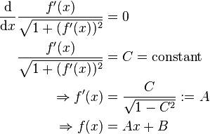
\frac{\partial L(x, y, y')}{\partial y'} = \frac{y'}{\sqrt{1 + y'^2}} \quad \text{and} \quad \frac{\partial L(x, y, y')}{\partial y} = 0.

By substituting these into the Euler–Lagrange equation, we obtain

\begin{align} \frac{\mathrm{d}}{\mathrm{d}x} \frac{f'(x)}{\sqrt{1 + (f'(x))^2}} &= 0 \\ \frac{f'(x)}{\sqrt{1 + (f'(x))^2}} &= C = \text{constant} \\ \Rightarrow f'(x)&= \frac{C}{\sqrt{1-C^2}} := A \\ \Rightarrow f(x) &= Ax + B \end{align}

that is, the function must have constant first derivative, and thus its graph is a straight line.

Variations for several functions, several variables, and higher derivatives

Single function of single variable with higher derivatives

The stationary values of the functional

I[f] = \int_{x_0}^{x_1} \mathcal{L}(x, f, f', f'', \dots, f^{(n)})~\mathrm{d}x ~;~~ f' := \cfrac{\mathrm{d}f}{\mathrm{d}x}, ~f'' := \cfrac{\mathrm{d}^2f}{\mathrm{d}x^2}, ~ f^{(n)} := \cfrac{\mathrm{d}^nf}{\mathrm{d}x^n}

can be obtained from the Euler–Lagrange equation^[4]

\cfrac{\partial \mathcal{L}}{\partial f} - \cfrac{\mathrm{d}}{\mathrm{d} x}\left(\cfrac{\partial \mathcal{L}}{\partial f'}\right) + \cfrac{\mathrm{d}^2}{\mathrm{d} x^2}\left(\cfrac{\partial \mathcal{L}}{\partial f''}\right) - \dots + (-1)^n \cfrac{\mathrm{d}^n}{\mathrm{d} x^n}\left(\cfrac{\partial \mathcal{L}}{\partial f^{(n)}}\right) = 0

under fixed boundary conditions for the function itself as well as for the first $n-1$ derivatives (i.e. for all $f^{(i)}, i \in \{0, ..., n-1\}$ ). The endpoint values of the highest derivative $f^{(n)}$ remain flexible.

Several functions of one variable

If the problem involves finding several functions ( $f_1, f_2, \dots, f_n$ ) of a single independent variable ( $x$ ) that define an extremum of the functional

I[f_1,f_2, \dots, f_n] = \int_{x_0}^{x_1} \mathcal{L}(x, f_1, f_2, \dots, f_n, f_1', f_2', \dots, f_n')~\mathrm{d}x ~;~~ f_i' := \cfrac{\mathrm{d}f_i}{\mathrm{d}x}

then the corresponding Euler–Lagrange equations are^[5]

\begin{align} \cfrac{\partial \mathcal{L}}{\partial f_i} - \cfrac{\mathrm{d}}{\mathrm{d}x}\left(\cfrac{\partial \mathcal{L}}{\partial f_i'}\right) = 0 \end{align}

Single function of several variables

A multi-dimensional generalization comes from considering a function on n variables. If Ω is some surface, then

I[f] = \int_{\Omega} \mathcal{L}(x_1, \dots , x_n, f, f_{x_1}, \dots , f_{x_n})\, \mathrm{d}\mathbf{x}\,\! ~;~~ f_{x_i} := \cfrac{\partial f}{\partial x_i}

is extremized only if f satisfies the partial differential equation

\frac{\partial \mathcal{L}}{\partial f} - \sum_{i=1}^{n} \frac{\partial}{\partial x_i} \frac{\partial \mathcal{L}}{\partial f_{x_i}} = 0. \,\!

When n = 2 and $\mathcal{L}$ is the energy functional, this leads to the soap-film minimal surface problem.

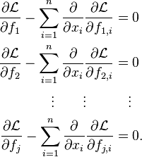
Several functions of several variables

If there are several unknown functions to be determined and several variables such that

I[f_1,f_2,\dots,f_m] = \int_{\Omega} \mathcal{L}(x_1, \dots , x_n, f_1, \dots, f_m, f_{1,1}, \dots , f_{1,n}, \dots, f_{m,1}, \dots, f_{m,n}) \, \mathrm{d}\mathbf{x}\,\! ~;~~ f_{j,i} := \cfrac{\partial f_j}{\partial x_i}

the system of Euler–Lagrange equations is^[4]

\begin{align} \frac{\partial \mathcal{L}}{\partial f_1} - \sum_{i=1}^{n} \frac{\partial}{\partial x_i} \frac{\partial \mathcal{L}}{\partial f_{1,i}} &= 0 \\ \frac{\partial \mathcal{L}}{\partial f_2} - \sum_{i=1}^{n} \frac{\partial}{\partial x_i} \frac{\partial \mathcal{L}}{\partial f_{2,i}} &= 0 \\ \vdots \qquad \vdots \qquad &\quad \vdots \\ \frac{\partial \mathcal{L}}{\partial f_j} - \sum_{i=1}^{n} \frac{\partial}{\partial x_i} \frac{\partial \mathcal{L}}{\partial f_{j,i}} &= 0. \end{align}

Single function of two variables with higher derivatives

If there is a single unknown function f to be determined that is dependent on two variables x₁ and x₂ and if the functional depends on higher derivatives of f up to n-th order such that

\begin{align} I[f] & = \int_{\Omega} \mathcal{L}(x_1, x_2, f, f_{,1}, f_{,2}, f_{,11}, f_{,12}, f_{,22}, \dots, f_{,22\dots 2})\, \mathrm{d}\mathbf{x} \\ & \qquad \quad f_{,i} := \cfrac{\partial f}{\partial x_i} \; , \quad f_{,ij} := \cfrac{\partial^2 f}{\partial x_i\partial x_j} \; , \;\; \dots \end{align}

then the Euler–Lagrange equation is^[4]

\begin{align} \frac{\partial \mathcal{L}}{\partial f} & - \frac{\partial}{\partial x_1}\left(\frac{\partial \mathcal{L}}{\partial f_{,1}}\right) - \frac{\partial}{\partial x_2}\left(\frac{\partial \mathcal{L}}{\partial f_{,2}}\right) + \frac{\partial^2}{\partial x_1^2}\left(\frac{\partial \mathcal{L}}{\partial f_{,11}}\right) + \frac{\partial^2}{\partial x_1\partial x_2}\left(\frac{\partial \mathcal{L}}{\partial f_{,12}}\right) + \frac{\partial^2}{\partial x_2^2}\left(\frac{\partial \mathcal{L}}{\partial f_{,22}}\right) \\ & - \dots + (-1)^n \frac{\partial^n}{\partial x_2^n}\left(\frac{\partial \mathcal{L}}{\partial f_{,22\dots 2}}\right) = 0 \end{align}

which can be represented shortly as:

\frac{\partial \mathcal{L}}{\partial f} +\sum_{i=1}^n (-1)^i \frac{\partial^i}{\partial x_{\mu_{1}}\dots \partial x_{\mu_{i}}} \left( \frac{\partial \mathcal{L} }{\partial f_{,\mu_1\dots\mu_i}}\right)=0

where $\mu_1 \dots \mu_i$ are indices that span the number of variables, that is they go from 1 to 2. Here summation over the $\mu_1 \dots \mu_i$ indices is implied according to Einstein notation.

Several functions of several variables with higher derivatives

If there is are p unknown functions f_i to be determined that are dependent on m variables x₁ ... x_m and if the functional depends on higher derivatives of the f_i up to n-th order such that

\begin{align} I[f_1,\ldots,f_p] & = \int_{\Omega} \mathcal{L}(x_1, \ldots, x_m; f_1,\ldots,f_p; f_{1,1},\ldots, f_{p,m}; f_{1,11},\ldots, f_{p,mm};\ldots; f_{p,m\ldots m})\, \mathrm{d}\mathbf{x} \\ & \qquad \quad f_{i,\mu} := \cfrac{\partial f_i}{\partial x_\mu} \; , \quad f_{i,\mu_1\mu_2} := \cfrac{\partial^2 f_i}{\partial x_{\mu_1}\partial x_{\mu_2}} \; , \;\; \dots \end{align}

where $\mu_1 \dots \mu_j$ are indices that span the number of variables, that is they go from 1 to m. Then the Euler–Lagrange equation is

\frac{\partial \mathcal{L}}{\partial f_i} +\sum_{j=1}^n (-1)^j \frac{\partial^j}{\partial x_{\mu_{1}}\dots \partial x_{\mu_{j}}} \left( \frac{\partial \mathcal{L} }{\partial f_{i,\mu_1\dots\mu_j}}\right)=0

where summation over the $\mu_1 \dots \mu_j$ is implied according to Einstein notation. This can be expressed more compactly as

\sum_{j=0}^n (-1)^j \partial_{ \mu_{1}\ldots \mu_{j} }^j \left( \frac{\partial \mathcal{L} }{\partial f_{i,\mu_1\dots\mu_j}}\right)=0

Generalization to Manifolds

Let $M$ be a smooth manifold, and let $C^\infty([a,b])$ denote the space of smooth functions $f:[a,b]\to M$ . Then, for functionals $S:C^\infty ([a,b])\to \mathbb{R}$ of the form

S[f]=\int_a^b (L\circ\dot{f})(t)\,\mathrm{d} t

where $L:TM\to\mathbb{R}$ is the Lagrangian, the statement $\mathrm{d} S_f=0$ is equivalent to the statement that, for all $t\in [a,b]$ , each coordinate frame trivialization $(x^i,X^i)$ of a neighborhood of $\dot{f}(t)$ yields the following $\dim M$ equations:

\forall i:\frac{\mathrm{d}}{\mathrm{d}t}\frac{\partial F}{\partial X^i}\bigg|_{\dot{f}(t)}=\frac{\partial F}{\partial x^i}\bigg|_{\dot{f}(t)}

Notes

↑ Fox, Charles (1987). An introduction to the calculus of variations. Courier Dover Publications. ISBN 978-0-486-65499-7.
↑ A short biography of Lagrange
↑ Courant & Hilbert 1953, p. 184
1 2 3 Courant, R; Hilbert, D (1953). Methods of Mathematical Physics. Vol. I (First English ed.). New York: Interscience Publishers, Inc. ISBN 978-0471504474.
↑ Weinstock, R., 1952, Calculus of Variations With Applications to Physics and Engineering, McGraw-Hill Book Company, New York.

References

Hazewinkel, Michiel, ed. (2001), "Lagrange equations (in mechanics)", Encyclopedia of Mathematics, Springer, ISBN 978-1-55608-010-4
Weisstein, Eric W., "Euler-Lagrange Differential Equation", MathWorld.
Calculus of Variations at PlanetMath.org.
Gelfand, Izrail Moiseevich (1963). Calculus of Variations. Dover. ISBN 0-486-41448-5.
Roubicek, T.: Calculus of variations. Chap.17 in: Mathematical Tools for Physicists. (Ed. M. Grinfeld) J. Wiley, Weinheim, 2014, ISBN 978-3-527-41188-7, pp.551-588.

This article is issued from Wikipedia - version of the Monday, February 08, 2016. The text is available under the Creative Commons Attribution/Share Alike but additional terms may apply for the media files.