Spline (mathematics)


In mathematics, a spline is a numeric function that is piecewise-defined by polynomial functions, and which possesses a high degree of smoothness at the places where the polynomial pieces connect (which are known as knots).[1][2]
In interpolating problems, spline interpolation is often preferred to polynomial interpolation because it yields similar results to interpolating with higher degree polynomials while avoiding instability due to Runge's phenomenon. In computer graphics, parametric curves whose coordinates are given by splines are popular because of the simplicity of their construction, their ease and accuracy of evaluation, and their capacity to approximate complex shapes through curve fitting and interactive curve design.
The most commonly used splines are cubic spline, i.e., of order 3—in particular, cubic B-spline, which is equivalent to C2 continuous composite Bézier curves.[3] They are common, in particular, in spline interpolation simulating the function of flat splines.
The term spline is adopted from the name of a flexible strip of metal commonly used by drafters to assist in drawing curved lines.[4]
Examples


A simple example of a quadratic spline (a spline of degree 2) is
for which  .
.
A simple example of a cubic spline is
as
and
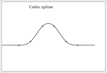
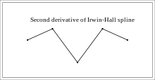
An example of using a cubic spline to create a bell shaped curve is the Irwin-Hall distribution polynomials:
History
Before computers were used, numerical calculations were done by hand. Functions such as the step function were used but polynomials were generally preferred. With the advent of computers, splines first replaced polynomials in interpolation, and then served in construction of smooth and flexible shapes in computer graphics.[5]
The word "spline" originally meant a thin wood or metal slat in East Anglian dialect. By 1895 it had come to mean a flexible ruler used to draw curves.[6] These splines were used in the aircraft and shipbuilding industries. For years ship designers had employed models to design hulls in small scale. The successful design was then plotted on graph paper and the key points of the plot were re-plotted on larger graph paper to full size. The thin wooden strips provided an interpolation of the key points into smooth curves. The strips would be held in place at the key points (using lead weights called "ducks"[7] (see Spline Ducks for illustration) or "dogs" or "rats"[8]) and between these points would assume shapes of minimum strain energy. In the foreword to Bartels et al. (1987),[7] Robin Forrest describes "lofting", a technique used in the British aircraft industry during World War II to construct templates for airplanes by passing thin wooden strips (called "splines") through points laid out on the floor of a large design loft.
It is commonly accepted that the first mathematical reference to splines is the 1946 paper by Schoenberg,[8] which is probably the first place that the word "spline" is used in connection with smooth, piecewise polynomial approximation. According to Forrest, one possible impetus for a mathematical model for this process was the potential loss of the critical design components for an entire aircraft should the loft be hit by an enemy bomb. This gave rise to "conic lofting", which used conic sections to model the position of the curve between the ducks. Conic lofting was replaced by what we would call splines in the early 1960s based on work by J. C. Ferguson[9] at Boeing and (somewhat later) by M. A. Sabin at British Aircraft Corporation.
The use of splines for modeling automobile bodies seems to have several independent beginnings. Credit is claimed on behalf of de Casteljau at Citroën, Pierre Bézier at Renault, and Birkhoff,[10] Garabedian, and de Boor at General Motors (see Birkhoff and de Boor, 1965),[11] all for work occurring in the very early 1960s or late 1950s. At least one of de Casteljau's papers was published, but not widely, in 1959. De Boor's work at General Motors resulted in a number of papers being published in the early 1960s, including some of the fundamental work on B-splines.[12]
Work was also being done at Pratt & Whitney Aircraft, where two of the authors of the first book-length treatment of splines (Ahlberg et al., 1967)[13] were employed; and the David Taylor Model Basin, by Feodor Theilheimer. The work at General Motors is detailed nicely in Birkhoff (1990) and Young (1997).[14] Davis (1997) summarizes some of this material.
Whittaker [15] derived a spline for smoothing data. He seems to be the first to propose balancing a measure of fit with a penalty term based on the sums-of-squares of the third differences of the function. He treats the penalty term as a prior distribution and estimates the spline through Bayes theorem.
Definition
A spline is a piecewise-polynomial real function
on an interval [a,b] composed of k subintervals ![[t_{i-1}, t_i]](../I/m/5ce2d2e0f7396e2cbbef6ec1bc107eaa.png) with
with
 .
.
The restriction of S to an interval i is a polynomial
![P_i: [t_{i-1}, t_i] \to \mathbb{R}](../I/m/548f8d10cc815f7342399e9fa2cdd8c1.png) ,
,
so that
The highest order of the polynomials  is said to be the order of the spline S. The spline is said to be uniform if all subintervals are of the same length, and non-uniform otherwise.[16]
The idea is to choose the polynomials in a way that guarantees sufficient smoothness of S. Specifically, for a spline of order n, S is required to be both continuous and continuously differentiable to order n-1 at the interior points  : for
: for  and
and 
 .
.
Derivation of a cubic spline interpolating between points
Spline interpolation is one of the most common uses of splines.
See also
- B-spline
- Biarc
- Discrete spline interpolation
- Perfect spline
- Smoothing spline
- T-Spline
- Spline wavelet
References
- ↑ Judd, Kenneth L. (1998). Numerical Methods in Economics. MIT Press. p. 225. ISBN 978-0-262-10071-7.
- ↑ Chen, Wai-Kai (2009). Feedback, Nonlinear, and Distributed Circuits. CRC Press. pp. 9–20. ISBN 978-1-4200-5881-9.
- ↑ An Introduction to Splines for Use in Computer Graphics and Geometric Modeling, p. 215, at Google Books
- ↑ Katz, Mitchell H. (2011). Multivariable Analysis: A Practical Guide for Clinicians and Public Health Researchers. Cambridge University Press. p. 82. ISBN 978-0-521-14107-9.
- ↑ Epperson (1998). "History of Splines". NA Digest 98 (26).
- ↑ "spline". Oxford English Dictionary (3rd ed.). Oxford University Press. September 2005. (Subscription or UK public library membership required.)
- 1 2 Bartels; Beatty; Barsky (1987). An Introduction to Splines for Use in Computer Graphics and Geometric Modeling.
- 1 2 Schoenberg (1946). "Contributions to the Problem of Approximation of Equidistant Data by Analytic Functions". Quart. Appl. Math. 4: 45–99 and 112–141.
- ↑ Ferguson, James C. (1964). "Multi-variable Curve Interpolation". J. ACM 11 (2): 221–228. doi:10.1145/321217.321225.
- ↑ Birkhoff (1990). "Fluid dynamics, reactor computations, and surface representation". In Nash, Steve. A History of Scientific Computation.
- ↑ Birkhoff; de Boor (1965). "Piecewise polynomial interpolation and approximation". In Garabedian, H. L. Proc. General Motors Symposium of 1964. New York and Amsterdam: Elsevier. pp. 164–190.
- ↑ Davis (1997). "B-splines and Geometric design". SIAM News 29 (5).
- ↑ Ahlberg; Nilson; Walsh (1967). The Theory of Splines and Their Applications.
- ↑ Young (1997). "Garrett Birkhoff and Applied Mathematics". Notices of the AMS 44 (11): 1446–1449.
- ↑ Whittaker, E. T. (1923). "On a new method of graduation". Proceedings of the Edinburgh Mathematical Society 41: 63–75.
- ↑ Fan, Jianqing & Yao, Qiwei (2005). "Spline Methods". Nonlinear time series: nonparametric and parametric methods. Springer. p. 247. ISBN 978-0-387-26142-3.
Further reading
- Smith, P. L. (1979). "Splines as a Useful and Convenient Statistical Tool". The American Statistician 33 (2): 57–62. doi:10.1080/00031305.1979.10482661.
- Stoer; Bulirsch (1980). Introduction to Numerical Analysis. Springer Science+Business Media. pp. 93–106. ISBN 0-387-90420-4.
- Chapra; Canale (2006). Numerical Methods for Engineers (5th ed.). Boston: McGraw-Hill. ISBN 0-07-124429-8.
External links
| Wikimedia Commons has media related to Splines. |
Theory
- Cubic Splines Module Prof. John H. Mathews California State University, Fullerton
- Spline Curves, Prof. Donald H. House Clemson University
- An Interactive Introduction to Splines, ibiblio.org
- Introduction to Splines, codeplea.com
Excel functions
- Open source Excel cubic spline User Defined Function
- SRS1 Cubic Spline for Excel - Free Excel cubic spline function (with utility to embed spline function code into any workbook)
Online utilities
- Visual, interactive comparison of various types of splines
- Online Cubic Spline Interpolation Utility
- Learning by Simulations Interactive simulation of various cubic splines
- Symmetrical Spline Curves, an animation by Theodore Gray, The Wolfram Demonstrations Project, 2007.
Computer code
- Notes, PPT, Mathcad, Maple, Mathematica, Matlab, Holistic Numerical Methods Institute
- various routines, NTCC
- Sisl: Opensource C-library for NURBS, SINTEF
- TinySpline: Opensource C-library for NURBS, B-Splines and Bezier Splines with bindings for various languages
- Closed Bezier Spline, C#, WPF, Oleg V. Polikarpotchkin
- Bezier Spline from 2D Points, C#, WPF, Oleg V. Polikarpotchkin


![S: [a,b]\to \mathbb{R}](../I/m/657900f76cf7e30d7258beca0a49f9ad.png)


