Conditional probability

Probability theory
Part of a series on Statistics

Probability axioms
Probability space Sample space Elementary event Event Random variable Probability measure
Complementary event Joint probability Marginal probability Conditional probability
Independence Conditional independence Law of total probability Law of large numbers Bayes' theorem Boole's inequality
Venn diagram Tree diagram

In probability theory, conditional probability is a measure of the probability of an event given that (by assumption, presumption, assertion or evidence) another event has occurred.^[1] If the event of interest is A and the event B is known or assumed to have occurred, "the conditional probability of A given B", or "the probability of A under the condition B", is usually written as P(A|B), or sometimes P_B(A). For example, the probability that any given person has a cough on any given day may be only 5%. But if we know or assume that the person has a cold, then they are much more likely to be coughing. The conditional probability of coughing given that you have a cold might be a much higher 75%.

The concept of conditional probability is one of the most fundamental and one of the most important concepts in probability theory.^[2] But conditional probabilities can be quite slippery and require careful interpretation.^[3] For example, there need not be a causal or temporal relationship between A and B.

P(A|B) may or may not be equal to P(A) (the unconditional probability of A). If P(A|B) = P(A), then events A and B are said to be independent. In such a case, having learned about the event B does not change our knowledge about the event A. Also, in general, P(A|B) (the conditional probability of A given B) is not equal to P(B|A). For example, if you have cancer you might have a 90% chance of testing positive for cancer. In this case what is being measured is that the if event B "having cancer" has occurred, the probability A - test is positive given that B having cancer occurred is 90%, P(A|B) = 90%. Alternatively, you can test positive for cancer but you may have only a 10% chance of actually having cancer because cancer is very rare. In this case what is being measured is the probability of the event B - having cancer given that the event A - test is positive has occurred, P(B|A) = 10%. Falsely equating the two probabilities causes various errors of reasoning such as the base rate fallacy. Conditional probabilities can be correctly reversed using Bayes' theorem.

Definition

Illustration of conditional probabilities with an Euler diagram. The unconditional probability P(A) = 0.52. However, the conditional probability P(A|B₁) = 1, P(A|B₂) = 0.75, and P(A|B₃) = 0.

On a tree diagram, branch probabilities are conditional on the event associated with the parent node.

Venn Pie Chart describing conditional probabilities

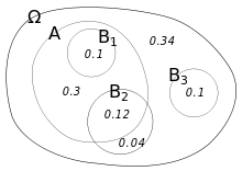
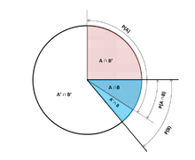
Conditioning on an event

Kolmogorov definition

Given two events A and B from the sigma-field of a probability space with P(B) > 0, the conditional probability of A given B is defined as the quotient of the probability of the joint of events A and B, and the probability of B:

P(A|B) = \frac{P(A \cap B)}{P(B)}

This may be visualized as restricting the sample space to B. The logic behind this equation is that if the outcomes are restricted to B, this set serves as the new sample space.

Note that this is a definition but not a theoretical result. We just denote the quantity $P(A\cap B)/P(B)$ as $P(A|B)$ and call it the conditional probability of A given B.

As an axiom of probability

Some authors, such as De Finetti, prefer to introduce conditional probability as an axiom of probability:

P(A \cap B) = P(A|B)P(B)

Although mathematically equivalent, this may be preferred philosophically; under major probability interpretations such as the subjective theory, conditional probability is considered a primitive entity. Further, this "multiplication axiom" introduces a symmetry with the summation axiom for mutually exclusive events:^[4]

P(A \cup B) = P(A) + P(B) - \cancelto0{P(A \cap B)}

Definition with σ-algebra

If P(B) = 0, then the simple definition of P(A|B) is undefined. However, it is possible to define a conditional probability with respect to a σ-algebra of such events (such as those arising from a continuous random variable).

For example, if X and Y are non-degenerate and jointly continuous random variables with density ƒ_X,Y(x, y) then, if B has positive measure,

P(X \in A \mid Y \in B) = \frac{\int_{y\in B}\int_{x\in A} f_{X,Y}(x,y)\,dx\,dy}{\int_{y\in B}\int_{x\in\Omega} f_{X,Y}(x,y)\,dx\,dy} .

The case where B has zero measure can only be dealt with directly in the case that B = {y₀}, representing a single point, in which case

P(X \in A \mid Y = y_0) = \frac{\int_{x\in A} f_{X,Y}(x,y_0)\,dx}{\int_{x\in\Omega} f_{X,Y}(x,y_0)\,dx} .

If A has measure zero then the conditional probability is zero. An indication of why the more general case of zero measure cannot be dealt with in a similar way can be seen by noting that the limit, as all δy_i approach zero, of

P(X \in A \mid Y \in \cup_i[y_i,y_i+\delta y_i]) \approxeq \frac{\sum_{i} \int_{x\in A} f_{X,Y}(x,y_i)\,dx\,\delta y_i}{\sum_{i}\int_{x\in\Omega} f_{X,Y}(x,y_i) \,dx\, \delta y_i} ,

depends on their relationship as they approach zero. See conditional expectation for more information.

Conditioning on a random variable

Conditioning on an event may be generalized to conditioning on a random variable. Let X be a random variable; we assume for the sake of presentation that X is discrete, that is, X takes on only finitely many values x. Let A be an event. The conditional probability of A given X is defined as the random variable, written P(A|X), that takes on the value

P(A\mid X=x)

whenever

X=x.

More formally:

P(A|X)(\omega)=P(A\mid X=X(\omega)) .

The conditional probability P(A|X) is a function of X, e.g., if the function g is defined as

g(x)= P(A\mid X=x)

then

P(A|X) =g\circ X

Note that P(A|X) and X are now both random variables. From the law of total probability, the expected value of P(A|X) is equal to the unconditional probability of A.

Example

Suppose that somebody secretly rolls two fair six-sided dice, and we must predict the outcome.

Let A be the value rolled on die 1
Let B be the value rolled on die 2

What is the probability that A = 2?

Table 1 shows the sample space of 36 outcomes

Clearly, A = 2 in exactly 6 of the 36 outcomes, thus P(A=2) = ⁶⁄₃₆ = ¹⁄₆.

Table 1
+	B=1	2	3	4	5	6
A=1	2	3	4	5	6	7
2	3	4	5	6	7	8
3	4	5	6	7	8	9
4	5	6	7	8	9	10
5	6	7	8	9	10	11
6	7	8	9	10	11	12

Suppose it is revealed that A+B ≤ 5

What is the probability A+B ≤ 5 ?

Table 2 shows that A+B ≤ 5 for exactly 10 of the same 36 outcomes, thus P(A+B ≤ 5) = ¹⁰⁄₃₆

Table 2
+	B=1	2	3	4	5	6
A=1	2	3	4	5	6	7
2	3	4	5	6	7	8
3	4	5	6	7	8	9
4	5	6	7	8	9	10
5	6	7	8	9	10	11
6	7	8	9	10	11	12

What is the probability that A = 2 given that A+B ≤ 5 ?

Table 3 shows that for 3 of these 10 outcomes, A = 2

Thus, the conditional probability P(A=2 | A+B ≤ 5) = ³⁄₁₀ = 0.3.

Table 3
+	B=1	2	3	4	5	6
A=1	2	3	4	5	6	7
2	3	4	5	6	7	8
3	4	5	6	7	8	9
4	5	6	7	8	9	10
5	6	7	8	9	10	11
6	7	8	9	10	11	12

Use in inference

In statistical inference, the conditional probability is an update of the probability of an event based on new information.^[3] Incorporating the new information can be done as follows ^[1]

Let A the event of interest be in the sample space, say (X,P).
The occurrence of the event A knowing that event B has or will have occurred, means the occurrence of A as it is restricted to B, i.e. $A \cap B$ .
Without the knowledge of the occurrence of B, the information about the occurrence of A would simply be P(A)
The probability of A knowing that event B has or will have occurred, will be the probability of $A \cap B$ compared with P(B), the probability B has occurred.
This results in P(A|B) = P(A $\cap$ B)/P(B) whenever P(B)>0 and 0 otherwise.

Note: This approach results in a probability measure that is consistent with the original probability measure and satisfies all the Kolmogorov Axioms. This conditional probability measure also could have resulted by assuming that the relative magnitude of the probability of A with respect to X will be preserved with respect to B (cf. a Formal Derivation below).

Note: The phraseology "evidence" or "information" is generally used in the Bayesian interpretation of probability. The conditioning event is interpreted as evidence for the conditioned event. That is, P(A) is the probability of A before accounting for evidence E, and P(A|E) is the probability of A after having accounted for evidence E or after having updated P(A). This is consistent with the frequentist interpretation, which presumably is the first definition given above.

Statistical independence

Main article: Independence (probability theory)

Events A and B are defined to be statistically independent if

P(A \cap B) = P(A) P(B).

If P(B) is not zero, then this is equivalent to the statement that

P(A|B) = P(A).

Similarly, if P(A) is not zero, then

P(B|A) = P(B).

is also equivalent. Although the derived forms may seem more intuitive, they are not the preferred definition as the conditional probabilities may be undefined, and the preferred definition is symmetrical in A and B.

Common fallacies

These fallacies should not be confused with Robert K. Shope's 1978 "conditional fallacy", which deals with counterfactual examples that beg the question.

Assuming conditional probability is of similar size to its inverse

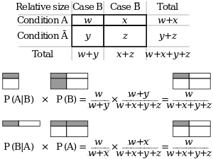
Main article: Confusion of the inverse

A geometric visualisation of Bayes' theorem. In the table, the values w, x, y and z give the relative weights of each corresponding condition and case. The figures denote the cells of the table involved in each metric, the probability being the fraction of each figure that is shaded. This shows that P(A|B) P(B) = P(B|A) P(A) i.e. P(A|B) = P(B|A) P(A)/P(B) . Similar reasoning can be used to show that P(Ā|B) = P(B|Ā) P(Ā)/P(B) etc.

In general, it cannot be assumed that P(A|B) ≈ P(B|A). This can be an insidious error, even for those who are highly conversant with statistics.^[5] The relationship between P(A|B) and P(B|A) is given by Bayes' theorem:

P(B|A) = \frac{P(A|B) P(B)}{P(A)}.

That is, P(A|B) ≈ P(B|A) only if P(B)/P(A) ≈ 1, or equivalently, P(A) ≈ P(B).

Alternatively, noting that A ∩ B = B ∩ A, and applying conditional probability:

P(A|B)P(B) = P(A \cap B) = P(B \cap A) = P(B|A)P(A)

Rearranging gives the result.

Assuming marginal and conditional probabilities are of similar size

In general, it cannot be assumed that P(A) ≈ P(A|B). These probabilities are linked through the law of total probability:

P(A) = \sum_n P(A \cap B_n) = \sum_n P(A|B_n)P(B_n)

where the events $(B_n)$ form a countable partition of $A$ .

This fallacy may arise through selection bias.^[6] For example, in the context of a medical claim, let S_C be the event that a sequela (chronic disease) S occurs as a consequence of circumstance (acute condition) C. Let H be the event that an individual seeks medical help. Suppose that in most cases, C does not cause S so P(S_C) is low. Suppose also that medical attention is only sought if S has occurred due to C. From experience of patients, a doctor may therefore erroneously conclude that P(S_C) is high. The actual probability observed by the doctor is P(S_C|H).

Over- or under-weighting priors

Not taking prior probability into account partially or completely is called base rate neglect. The reverse, insufficient adjustment from the prior probability is conservatism.

Formal derivation

Formally, P(A|B) is defined as the probability of A according to a new probability function on the sample space, such that outcomes not in B have probability 0 and that it is consistent with all original probability measures.^[7]^[8]

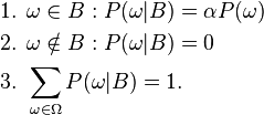
Let Ω be a sample space with elementary events {ω}. Suppose we are told the event B ⊆ Ω has occurred. A new probability distribution (denoted by the conditional notation) is to be assigned on {ω} to reflect this. For events in B, it is reasonable to assume that the relative magnitudes of the probabilities will be preserved. For some constant scale factor α, the new distribution will therefore satisfy:

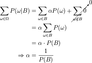
\begin{align} &\text{1. }\omega \in B : P(\omega|B) = \alpha P(\omega) \\ &\text{2. }\omega \notin B : P(\omega|B) = 0 \\ &\text{3. }\sum_{\omega \in \Omega} {P(\omega|B)} = 1. \end{align}

Substituting 1 and 2 into 3 to select α:

\begin{align} \sum_{\omega \in \Omega} {P(\omega | B)} &= \sum_{\omega \in B} {\alpha P(\omega)} + \cancelto{0}{\sum_{\omega \notin B} 0} \\ &= \alpha \sum_{\omega \in B} {P(\omega)} \\ &= \alpha \cdot P(B) \\ \Rightarrow \alpha &= \frac{1}{P(B)} \end{align}

So the new probability distribution is

\begin{align} \text{1. }\omega \in B&: P(\omega|B) = \frac{P(\omega)}{P(B)} \\ \text{2. }\omega \notin B&: P(\omega| B) = 0 \end{align}

Now for a general event A,

\begin{align} P(A|B) &= \sum_{\omega \in A \cap B} {P(\omega | B)} + \cancelto{0}{\sum_{\omega \in A \cap B^c} P(\omega|B)} \\ &= \sum_{\omega \in A \cap B} {\frac{P(\omega)}{P(B)}} \\ &= \frac{P(A \cap B)}{P(B)} \end{align}

References

1 2 Gut, Allan (2013). Probability: A Graduate Course (Second ed.). New York, NY: Springer. ISBN 978-1-4614-4707-8.
↑ Ross, Sheldon (2010). A First Course in Probability (8th ed.). Pearson Prentice Hall. ISBN 978-0-13-603313-4.
1 2 Casella, George; Berger, Roger L. (2002). Statistical Inference. Duxbury Press. ISBN 0-534-24312-6.
↑ Gillies, Donald (2000); "Philosophical Theories of Probability"; Routledge; Chapter 4 "The subjective theory"
↑ Paulos, J.A. (1988) Innumeracy: Mathematical Illiteracy and its Consequences, Hill and Wang. ISBN 0-8090-7447-8 (p. 63 et seq.)
↑ Thomas Bruss, F; Der Wyatt Earp Effekt; Spektrum der Wissenschaft; March 2007
↑ George Casella and Roger L. Berger (1990), Statistical Inference, Duxbury Press, ISBN 0-534-11958-1 (p. 18 et seq.)
↑ Grinstead and Snell's Introduction to Probability, p. 134

External links

Weisstein, Eric W., "Conditional Probability", MathWorld.
F. Thomas Bruss Der Wyatt-Earp-Effekt oder die betörende Macht kleiner Wahrscheinlichkeiten (in German), Spektrum der Wissenschaft (German Edition of Scientific American), Vol 2, 110–113, (2007).
Visual explanation of conditional probability

This article is issued from Wikipedia - version of the Monday, February 15, 2016. The text is available under the Creative Commons Attribution/Share Alike but additional terms may apply for the media files.