Clenshaw algorithm

In numerical analysis, the Clenshaw algorithm,^[1] also called Clenshaw summation,^[2] is a recursive method to evaluate a linear combination of Chebyshev polynomials. It is a generalization of Horner's method for evaluating a linear combination of monomials.

It generalizes to more than just Chebyshev polynomials; it applies to any class of functions that can be defined by a three-term recurrence relation.^[3]

Clenshaw algorithm

In full generality, the Clenshaw algorithm computes the weighted sum of a finite series of functions $\phi_k(x)$ :

S(x) = \sum_{k=0}^n a_k \phi_k(x)

where $\phi_k,\; k=0, 1, \ldots$ is a sequence of functions that satisfy the linear recurrence relation

\phi_{k+1}(x) = \alpha_k(x)\,\phi_k(x) + \beta_k(x)\,\phi_{k-1}(x),

where the coefficients $\alpha_k(x)$ and $\beta_k(x)$ are known in advance.

The algorithm is most useful when $\phi_k(x)$ are functions that are complicated to compute directly, but $\alpha_k(x)$ and $\beta_k(x)$ are particularly simple. In the most common applications, $\alpha(x)$ does not depend on $k$ , and $\beta$ is a constant that depends on neither $x$ nor $k$ .

To perform the summation for given series of coefficients $a_0, \ldots, a_n$ , compute the values $b_k(x)$ by the "reverse" recurrence formula:

\begin{align} b_{n+1}(x) &= b_{n+2}(x) = 0, \\ b_k(x) &= a_k + \alpha_k(x)\,b_{k+1}(x) + \beta_{k+1}(x)\,b_{k+2}(x). \end{align}

Note that this computation makes no direct reference to the functions $\phi_k(x)$ . After computing $b_2(x)$ and $b_1(x)$ , the desired sum can be expressed in terms of them and the simplest functions $\phi_0(x)$ and $\phi_1(x)$ :

S(x) = \phi_0(x)\,a_0 + \phi_1(x)\,b_1(x) + \beta_1(x)\,\phi_0(x)\,b_2(x).

See Fox and Parker^[4] for more information and stability analyses.

Examples

Horner as a special case of Clenshaw

A particularly simple case occurs when evaluating a polynomial of the form

S(x) = \sum_{k=0}^n a_k x^k

The functions are simply

\begin{align} \phi_0(x) &= 1, \\ \phi_k(x) &= x^k = x\phi_{k-1}(x) \end{align}

and are produced by the recurrence coefficients $\alpha(x) = x$ and $\beta = 0$ .

In this case, the recurrence formula to compute the sum is

b_k(x) = a_k + x b_{k+1}(x)

and, in this case, the sum is simply

S(x) = a_0 + x b_1(x) = b_0(x)

which is exactly the usual Horner's method.

Special case for Chebyshev series

Consider a truncated Chebyshev series

p_n(x) = a_0 + a_1T_1(x) + a_2T_2(x) + \cdots + a_nT_n(x).

The coefficients in the recursion relation for the Chebyshev polynomials are

\alpha(x) = 2x, \quad \beta = -1,

with the initial conditions

T_0(x) = 1, \quad T_1(x) = x.

Thus, the recurrence is

b_k(x) = a_k + 2xb_{k+1}(x) - b_{k+2}(x)

and the final sum is

p_n(x) = a_0 + xb_1(x) - b_2(x).

One way to evaluate this is to continue the recurrence one more step, and compute

b_0(x) = 2a_0 + 2xb_1(x) - b_2(x),

(note the doubled a₀ coefficient) followed by

p_n(x) = \frac{1}{2}\left[b_0(x) - b_2(x)\right].

Meridian arc length on the ellipsoid

Clenshaw summation is extensively used in geodetic applications.^[2] A simple application is summing the trigonometric series to compute the meridian arc distance on the surface of an ellipsoid. These have the form

m(\theta) = C_0\,\theta + C_1\sin \theta + C_2\sin 2\theta + \cdots + C_n\sin n\theta.

Leaving off the initial $C_0\,\theta$ term, the remainder is a summation of the appropriate form. There is no leading term because $\phi_0(\theta) = \sin 0\theta = \sin 0 = 0$ .

The recurrence relation for $\sin k\theta$ is

\sin (k+1)\theta = 2 \cos\theta \sin k\theta - \sin (k-1)\theta

making the coefficients in the recursion relation

\alpha_k(\theta) = 2\cos\theta, \quad \beta_k = -1.

and the evaluation of the series is given by

\begin{align} b_{n+1}(\theta) &= b_{n+2}(\theta) = 0, \\ b_k(\theta) &= C_k + 2\cos \theta \,b_{k+1}(\theta) - b_{k+2}(\theta),\quad\mathrm{for\ } n\ge k \ge 1. \end{align}

The final step is made particularly simple because $\phi_0(\theta) = \sin 0 = 0$ , so the end of the recurrence is simply $b_1(\theta)\sin(\theta)$ ; the $C_0\,\theta$ term is added separately:

m(\theta) = C_0\,\theta + b_1(\theta)\sin \theta.

Note that the algorithm requires only the evaluation of two trigonometric quantities $\cos \theta$ and $\sin \theta$ .

Difference in meridian arc lengths

Sometimes it necessary to compute the difference of two meridian arcs in a way that maintains high relative accuracy. This is accomplished by using trigonometric identities to write

m(\theta_1)-m(\theta_2) = \sum_{k=1}^n 2 C_k \sin\bigl({\textstyle\frac12}k(\theta_1-\theta_2)\bigr) \cos\bigl({\textstyle\frac12}k(\theta_1+\theta_2)\bigr).

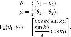
Clenshaw summation can be applied in this case^[5] provided we simultaneously compute $m(\theta_1)+m(\theta_2)$ and perform a matrix summation,

\mathsf M(\theta_1,\theta_2) = \begin{bmatrix} (m(\theta_1) + m(\theta_2)) / 2\\ (m(\theta_1) - m(\theta_2)) / (\theta_1 - \theta_2) \end{bmatrix} = C_0 \begin{bmatrix}\mu\\1\end{bmatrix} + \sum_{k=1}^n C_k \mathsf F_k(\theta_1,\theta_2),

where

\begin{align} \delta &= {\textstyle\frac12}(\theta_1-\theta_2), \\ \mu &= {\textstyle\frac12}(\theta_1+\theta_2), \\ \mathsf F_k(\theta_1,\theta_2) &= \begin{bmatrix} \cos k \delta \sin k \mu\\ \displaystyle\frac{\sin k \delta}\delta \cos k \mu \end{bmatrix}. \end{align}

The first element of $\mathsf M(\theta_1,\theta_2)$ is the average value of $m$ and the second element is the average slope. $\mathsf F_k(\theta_1,\theta_2)$ satisfies the recurrence relation

\mathsf F_{k+1}(\theta_1,\theta_2) = \mathsf A(\theta_1,\theta_2) \mathsf F_k(\theta_1,\theta_2) - \mathsf F_{k-1}(\theta_1,\theta_2),

where

\mathsf A(\theta_1,\theta_2) = 2\begin{bmatrix} \cos \delta \cos \mu & -\delta\sin \delta \sin \mu \\ - \displaystyle\frac{\sin \delta}\delta \sin \mu & \cos \delta \cos \mu \end{bmatrix}

takes the place of $\alpha$ in the recurrence relation, and $\beta=-1$ . The standard Clenshaw algorithm can now be applied to yield

\begin{align} \mathsf B_{n+1} &= \mathsf B_{n+2} = \mathsf 0, \\ \mathsf B_k &= C_k \mathsf I + \mathsf A \mathsf B_{k+1} - \mathsf B_{k+2}, \qquad\mathrm{for\ } n\ge k \ge 1,\\ \mathsf M(\theta_1,\theta_2) &= C_0 \begin{bmatrix}\mu\\1\end{bmatrix} + \mathsf B_1 \mathsf F_1(\theta_1,\theta_2), \end{align}

where $\mathsf B_k$ are 2×2 matrices. Finally we have

\frac{m(\theta_1) - m(\theta_2)}{\theta_1 - \theta_2} = \mathsf M_2(\theta_1, \theta_2).

This technique can be used in the limit $\theta_2 = \theta_1 = \mu$ and $\delta = 0\,$ to simultaneously compute $m(\mu)$ and the derivative $dm(\mu)/d\mu$ , provided that, in evaluating $\mathsf F_1$ and $\mathsf A$ , we take $\lim_{\delta\rightarrow0}(\sin \delta)/\delta = 1$ .

References

↑ Clenshaw, C. W. (July 1955). "A note on the summation of Chebyshev series". Mathematical Tables and other Aids to Computation 9 (51): 118–110. doi:10.1090/S0025-5718-1955-0071856-0. ISSN 0025-5718. Note that this paper is written in terms of the Shifted Chebyshev polynomials of the first kind $T^*_n(x) = T_n(2x-1)$ .
1 2 Tscherning, C. C.; Poder, K. (1982), "Some Geodetic applications of Clenshaw Summation" (PDF), Bolletino di Geodesia e Scienze Affini 41 (4): 349–375
↑ Press, WH; Teukolsky, SA; Vetterling, WT; Flannery, BP (2007), "Section 5.4.2. Clenshaw's Recurrence Formula", Numerical Recipes: The Art of Scientific Computing (3rd ed.), New York: Cambridge University Press, ISBN 978-0-521-88068-8
↑ Fox, Leslie; Parker, Ian B. (1968), Chebyshev Polynomials in Numerical Analysis, Oxford University Press, ISBN 0-19-859614-6
↑ Karney, C. F. F. (2014), Clenshaw evaluation of differenced sums

This article is issued from Wikipedia - version of the Monday, August 31, 2015. The text is available under the Creative Commons Attribution/Share Alike but additional terms may apply for the media files.

Clenshaw algorithm