Bayes linear statistics
Bayes linear statistics is a subjectivist statistical methodology and framework. Traditional subjective Bayesian analysis is based upon fully specified probability distributions, which are very difficult to specify at the necessary level of detail. Bayes linear analysis attempts to solve this problem by developing theory and practise for using partially specified probability models. Bayes linear in its current form has been primarily developed by Michael Goldstein. Mathematically and philosophically it extends Bruno de Finetti's Operational Subjective approach to probability and statistics.
Consider first a traditional Bayesian Analysis where you expect to shortly know D and you would like to know more about some other observable B. In the traditional Bayesian approach it is required that every possible outcome is enumerated i.e. every possible outcome is the cross product of the partition of a set of B and D. If represented on a computer where B requires n bits and D m bits then the number of states required is 2n+m. The first step to such an analysis is to determine a persons subjective probabilities e.g. by asking about their betting behaviour for each of these outcomes. When we learn D conditional probabilities for B are determined by the application of Bayes' rule.
Practitioners of subjective Bayesian statistics routinely analyse datasets where the size of this set is large enough that subjective probabilities cannot be meaningfully determined for every element of D × B. This is normally accomplished by assuming exchangeability and then the use of parameterized models with prior distributions over parameters and appealing to the de Finetti's theorem to justify that this produces valid operational subjective probabilities over D × B. The difficulty with such an approach is that the validity of the statistical analysis requires that the subjective probabilities are a good representation of an individual's beliefs however this method results in a very precise specification over D × B and it is often difficult to articulate what it would mean to adopt these belief specifications.
In contrast to the traditional Bayesian paradigm Bayes linear statistics following de Finetti uses Prevision or subjective expectation as a primitive, probability is then defined as the expectation of an indicator variable. Instead of specifying a subjective probability for every element in the partition D × B the analyst specifies subjective expectations for just a few quantities that they are interested in or feel knowledgeable about. Then instead of conditioning an adjusted expectation is computed by a rule that is a generalization of Bayes' rule that is based upon expectation.
The use of the word linear in the title refers to de Finetti's arguments that probability theory is a linear theory (de Finetti argued against the more common measure theory approach).
Example
In Bayes linear statistics, the probability model is only partially specified, and it is not possible to calculate conditional probability by Bayes' rule. Instead Bayes linear suggests the calculation of an Adjusted Expectation.
To conduct a Bayes linear analysis it is necessary to identify some values that you expect to know shortly by making measurements D and some future value which you would like to know B. Here D refers to a vector containing data and B to a vector containing quantities you would like to predict. For the following example B and D are taken to be two-dimensional vectors i.e.
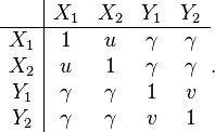
In order to specify a Bayes linear model it is necessary to supply expectations for the vectors B and D, and to also specify the correlation between each component of B and each component of D.
For example the expectations are specified as:
and the covariance matrix is specified as :
The repetition in this matrix, has some interesting implications to be discussed shortly.
An adjusted expectation is a linear estimator of the form
where  and
and  are chosen to minimise the prior expected loss for the observations i.e.
  in this case. That is for
where
are chosen in order to minimise the prior expected loss in estimating 
In general the adjusted expectation is calculated with
Setting  to minimise
From a proof provided in (Goldstein and Wooff 2007) it can be shown that:
For the case where Var(D) is not invertible the Moore–Penrose pseudoinverse should be used instead.
Furthermore, the adjusted variance of the variable  after observing the data
  is given by
See also
External links
References
- Goldstein, M. (1981) Revising Previsions: a Geometric Interpretation (with Discussion). Journal of the Royal Statistical Society, Series B, 43(2), 105-130
- Goldstein, M. (2006) Subjectivism principles and practice. Bayesian Analysis]
- Michael Goldstein, David Wooff (2007) Bayes Linear Statistics, Theory & Methods, Wiley. ISBN 978-0-470-01562-9
- de Finetti, B. (1931) "Probabilism: A Critical Essay on the Theory of Probability and on the Value of Science," (translation of 1931 article) in Erkenntnis, volume 31, September 1989. The entire double issue is devoted to de Finetti's philosophy of probability.
- de Finetti, B. (1937) “La Prévision: ses lois logiques, ses sources subjectives,” Annales de l'Institut Henri Poincaré,
- - "Foresight: its Logical Laws, Its Subjective Sources," (translation of the 1937 article in French) in H. E. Kyburg and H. E. Smokler (eds), Studies in Subjective Probability, New York: Wiley, 1964.
- de Finetti, B. (1974) Theory of Probability, (translation by A Machi and AFM Smith of 1970 book) 2 volumes, New York: Wiley, 1974-5.


![E([Y_1 - c_0 - c_1X_1 - c_2X_2]^2)\,](../I/m/dc20a48c9f2b163bbb3bedc3f52ad748.png)


![E\left(\left[X-\sum^k_{i=0}h_iD_i\right]^2\right).](../I/m/7314856d491c7bb97d9b7a1581a87894.png)

