Young's modulus
_Snapback_to_reality_(6283432546).jpg)
Young's modulus, also known as the tensile modulus or elastic modulus, is a measure of the stiffness of an elastic material and is a quantity used to characterize materials. It is defined as the ratio of the stress (force per unit area) along an axis to the strain (ratio of deformation over initial length) along that axis in the range of stress in which Hooke's law holds.[1]
Young's modulus is the most common elastic modulus, sometimes called the modulus of elasticity, but there are other elastic moduli such as the bulk modulus and the shear modulus.
It is named after the 19th-century British scientist Thomas Young. However, the concept was developed in 1727 by Leonhard Euler, and the first experiments that used the concept of Young's modulus in its current form were performed by the Italian scientist Giordano Riccati in 1782, pre-dating Young's work by 25 years.[2]
A material whose Young's modulus is very high is rigid. Do not confuse:
- rigidity and strength: the strength of material is characterized by its yield strength and / or its tensile strength;
- rigidity and stiffness: the beam stiffness (for example) depends on its Young's modulus but also on the ratio of its section to its length. The rigidity characterises the materials (it is an intensive property) while the stiffness regards products and constructions (it is an extensive property): a massive mechanical plastic part can be much stiffer than a steel spring;
- rigidity and hardness: the hardness of a material defines its relative resistance that its surface opposes to the penetration of a harder body.
- rigidity and toughness: toughness is the amount of energy that a material can absorb before fracturing when subjected to strain.
Units
Young's modulus is the ratio of stress (which has units of pressure) to strain (which is dimensionless), and so Young's modulus has units of pressure. Its SI unit is therefore the pascal (Pa or N/m2 or m−1·kg·s−2). The practical units used are megapascals (MPa or N/mm2) or gigapascals (GPa or kN/mm2). In United States customary units, it is expressed as pounds (force) per square inch (psi). The abbreviation ksi refers to "kips per square inch", or thousands of psi.
Usage
The Young's modulus enables the calculation of the change in the dimension of a bar made of an isotropic elastic material under tensile or compressive loads. For instance, it predicts how much a material sample extends under tension or shortens under compression. The Young's modulus directly applies to cases uniaxial stress, that is tensile or compressive stress in one direction and no stress in the other directions. Young's modulus is also used in order to predict the deflection that will occur in a statically determinate beam when a load is applied at a point in between the beam's supports. Other elastic calculations usually require the use of one additional elastic property, such as the shear modulus, bulk modulus or Poisson's ratio. Any two of these parameters are sufficient to fully describe elasticity in an isotropic material.
Linear versus non-linear
The Young's modulus represents the factor of proportionality in Hooke's law, which relates the stress and the strain. However, Hooke's law is only valid under the assumption of an elastic and linear response. Any real material will eventually fail and break when stretched over a very large distance or with a very large force; however all solid materials exhibit Hookean behavior for small enough strains or stresses. If the range over which Hooke's law is valid is large enough compared to the typical stress that one expects to apply to the material, the material is said to be linear. Otherwise (if the typical stress one would apply is outside the linear range) the material is said to be non-linear.
Steel, carbon fiber and glass among others are usually considered linear materials, while other materials such as rubber and soils are non-linear. However, this is not an absolute classification: if very small stresses or strains are applied to a non-linear material, the response will be linear, but if very high stress or strain is applied to a linear material, the linear theory will not be enough. For example, as the linear theory implies reversibility, it would be absurd to use the linear theory to describe the failure of a steel bridge under a high load; although steel is a linear material for most applications, it is not in such a case of catastrophic failure.
In solid mechanics, the slope of the stress–strain curve at any point is called the tangent modulus. It can be experimentally determined from the slope of a stress–strain curve created during tensile tests conducted on a sample of the material. The tangent modulus of the initial, linear portion of a stress–strain curve is called Young's modulus.
Directional materials
Young's modulus is not always the same in all orientations of a material. Most metals and ceramics, along with many other materials, are isotropic, and their mechanical properties are the same in all orientations. However, metals and ceramics can be treated with certain impurities, and metals can be mechanically worked to make their grain structures directional. These materials then become anisotropic, and Young's modulus will change depending on the direction of the force vector. Anisotropy can be seen in many composites as well. For example, carbon fiber has much higher Young's modulus (is much stiffer) when force is loaded parallel to the fibers (along the grain). Other such materials include wood and reinforced concrete. Engineers can use this directional phenomenon to their advantage in creating structures.
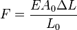
Calculation
Young's modulus, E, can be calculated by dividing the tensile stress by the extensional strain in the elastic (initial, linear) portion of the stress–strain curve:

where
- E is the Young's modulus (modulus of elasticity)
- F is the force exerted on an object under tension;
- A0 is the original cross-sectional area through which the force is applied;
- ΔL is the amount by which the length of the object changes;
- L0 is the original length of the object.
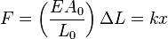
Force exerted by stretched or contracted material
The Young's modulus of a material can be used to calculate the force it exerts under specific strain.
where F is the force exerted by the material when contracted or stretched by ΔL.
Hooke's law can be derived from this formula, which describes the stiffness of an ideal spring:
where it comes in saturation
 and
and 
Elastic potential energy
The elastic potential energy stored is given by the integral of this expression with respect to L:

where Ue is the elastic potential energy.
The elastic potential energy per unit volume is given by:
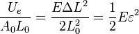 , where
  is the strain in the material.M
This formula can also be expressed as the integral of Hooke's law:

Relation among elastic constants
For homogeneous isotropic materials simple relations exist between elastic constants (Young's modulus E, shear modulus G, bulk modulus K, and Poisson's ratio ν) that allow calculating them all as long as two are known:

Approximate values

Young's modulus can vary somewhat due to differences in sample composition and test method. The rate of deformation has the greatest impact on the data collected, especially in polymers. The values here are approximate and only meant for relative comparison.
| Material | GPa | psi |
|---|---|---|
| Rubber (small strain) | 0.01–0.1[3] | 1,450–14,503 |
| Low density polyethylene[4] | 0.11–0.45 | 16,000–65,000 |
| Diatom frustules (largely silicic acid)[5] | 0.35–2.77 | 50,000–400,000 |
| PTFE (Teflon) | 0.5 [3] | 75,000 |
| HDPE | 0.8 | 116,000 |
| Bacteriophage capsids[6] | 1–3 | 150,000–435,000 |
| Polypropylene | 1.5–2[3] | 218,000–290,000 |
| Polyethylene terephthalate (PET) | 2–2.7[3] | 290,000–390,000 |
| Nylon | 2–4 | 290,000–580,000 |
| Polystyrene | 3–3.5[3] | 440,000–510,000 |
| Medium-density fiberboard (MDF)[7] | 4 | 580,000 |
| Oak wood (along grain) | 11[3] | 1.60×10⁶ |
| Human Cortical Bone[8] | 14 | 2.03×10⁶ |
| Glass-reinforced polyester matrix [9] | 17.2 | 2.49×10⁶ |
| Aromatic peptide nanotubes [10][11] | 19–27 | 2.76×10⁶–3.92×10⁶ |
| High-strength concrete | 30[3] | 4.35×10⁶ |
| Carbon fiber reinforced plastic (50/50 fibre/matrix, biaxial fabric) | 30–50[12] | 4.35×10⁶ – 7.25×10⁶ |
| Hemp fiber [13] | 35 | 5.08×10⁶ |
| Magnesium metal (Mg) | 45[3] | 6.53×10⁶ |
| Glass (see chart) | 50–90[3] | 7.25×10⁶ – 13.1×10⁶ |
| Flax fiber [14] | 58 | 8.41×10⁶ |
| Aluminum | 69[3] | 10.0×10⁶ |
| Mother-of-pearl (nacre, largely calcium carbonate) [15] | 70 | 10.2×10⁶ |
| Aramid[16] | 70.5–112.4 | 10.2×10⁶ – 16.3×10⁶ |
| Tooth enamel (largely calcium phosphate)[17] | 83 | 12.0×10⁶ |
| Stinging nettle fiber [18] | 87 | 12.6×10⁶ |
| Bronze | 96–120[3] | 13.9×10⁶ – 17.4×10⁶ |
| Brass | 100–125[3] | 14.5×10⁶ – 18.1×10⁶ |
| Titanium (Ti) | 110.3 | 16.0×10⁶[3] |
| Titanium alloys | 105–120[3] | 15.0×10⁶ – 17.5×10⁶ |
| Copper (Cu) | 117 | 17.0×10⁶ |
| Carbon fiber reinforced plastic (70/30 fibre/matrix, unidirectional, along grain)[19] | 181 | 26.3×10⁶ |
| Silicon Single crystal, different directions [20][21] | 130–185 | 18.9×10⁶ – 26.8×10⁶ |
| Wrought iron | 190–210[3] | 27.6×10⁶ – 30.5×10⁶ |
| Steel (ASTM-A36) | 200[3] | 29.0×10⁶ |
| polycrystalline Yttrium iron garnet (YIG)[22] | 193 | 28.0×10⁶ |
| single-crystal Yttrium iron garnet (YIG)[23] | 200 | 29.0×10⁶ |
| Aromatic peptide nanospheres [24] | 230–275 | 33.4×10⁶ – 39.9×10⁶ |
| Beryllium (Be)[25] | 287 | 41.6×10⁶ |
| Molybdenum (Mo) | 329 - 330 [3] [26] [27] | 47.7×10⁶–47.9×10⁶ |
| Tungsten (W) | 400 – 410 [3] | 58×106–59×106 |
| Silicon carbide (SiC) | 450 [3] | 65×106 |
| Tungsten carbide (WC) | 450 – 650 [3] | 65×106–94×106 |
| Osmium (Os) | 525 - 562 [28] | 76.1×10⁶–81.5×10⁶ |
| Single-walled carbon nanotube | 1,000 + [29][30] | 150×106 + |
| Graphene | 1,050[31] | 152×106 |
| Diamond (C) | 1,050 - 1210[32] | 152×106–175×106 |
| Carbyne (C)[33] | 32,100[34] | 4.66×10⁹ |
See also
- Deflection
- Deformation
- Hardness
- Hooke's law
- Shear modulus
- Bulk Modulus
- Bending stiffness
- Impulse excitation technique
- Toughness
- Yield (engineering)
- List of materials properties
References
- ↑ IUPAC, Compendium of Chemical Terminology, 2nd ed. (the "Gold Book") (1997). Online corrected version: (2006–) "modulus of elasticity (Young's modulus), E".
- ↑ The Rational Mechanics of Flexible or Elastic Bodies, 1638–1788: Introduction to Leonhardi Euleri Opera Omnia, vol. X and XI, Seriei Secundae. Orell Fussli.
- ↑ 3.0 3.1 3.2 3.3 3.4 3.5 3.6 3.7 3.8 3.9 3.10 3.11 3.12 3.13 3.14 3.15 3.16 3.17 3.18 3.19 "Elastic Properties and Young Modulus for some Materials". The Engineering ToolBox. Retrieved 2012-01-06.
- ↑ "Overview of materials for Low Density Polyethylene (LDPE), Molded". Matweb. Retrieved Feb 7, 2013.
- ↑ Subhash G, Yao S, Bellinger B, Gretz MR. (2005). "Investigation of mechanical properties of diatom frustules using nanoindentation". J Nanosci Nanotechnol. 5 (1): 50–6. doi:10.1166/jnn.2005.006. PMID 15762160.
- ↑ Ivanovska IL, de Pablo PJ, Sgalari G, MacKintosh FC, Carrascosa JL, Schmidt CF, Wuite GJL (2004). "Bacteriophage capsids: Tough nanoshells with complex elastic properties". Proc Nat Acad Sci USA. 101 (20): 7600–5. Bibcode:2004PNAS..101.7600I. doi:10.1073/pnas.0308198101. PMC 419652. PMID 15133147.
- ↑ Material Properties Data: Medium Density Fiberboard (MDF)
- ↑ Rho, JY (1993). "Young's modulus of trabecular and cortical bone material: ultrasonic and microtensile measurements". Journal of Biomechanics 26 (2): 111–119. doi:10.1016/0021-9290(93)90042-d.
- ↑ Polyester Matrix Composite reinforced by glass fibers (Fiberglass). [SubsTech] (2008-05-17). Retrieved on 2011-03-30.
- ↑ Kol, N. et al. (June 8, 2005). "Self-Assembled Peptide Nanotubes Are Uniquely Rigid Bioinspired Supramolecular Structures". Nano Letters 5 (7): 1343–1346. Bibcode:2005NanoL...5.1343K. doi:10.1021/nl0505896.
- ↑ Niu, L. et al. (June 6, 2007). "Using the Bending Beam Model to Estimate the Elasticity of Diphenylalanine Nanotubes". Langmuir 23 (14): 7443–7446. doi:10.1021/la7010106.
- ↑ E-G-nu.htm "Composites Design and Manufacture (BEng) – MATS 324".
- ↑ Nabi Saheb, D.; Jog, JP. (1999). "Natural fibre polymer composites: a review". Advances in Polymer Technology 18 (4): 351–363. doi:10.1002/(SICI)1098-2329(199924)18:4<351::AID-ADV6>3.0.CO;2-X.
- ↑ Bodros, E. (2002). "Analysis of the flax fibres tensile behaviour and analysis of the tensile stiffness increase". Composite Part A 33 (7): 939–948. doi:10.1016/S1359-835X(02)00040-4.
- ↑ A. P. Jackson,J. F. V. Vincent and R. M. Turner (1988). "The Mechanical Design of Nacre". Proceedings of the Royal Society B 234 (1277): 415–440. Bibcode:1988RSPSB.234..415J. doi:10.1098/rspb.1988.0056.
- ↑ DuPont (2001). "Kevlar Technical Guide". p. 9.
- ↑ M. Staines, W. H. Robinson and J. A. A. Hood (1981). "Spherical indentation of tooth enamel". Journal of Materials Science 16 (9): 2551–2556. doi:10.1007/bf01113595.
- ↑ Bodros, E.; Baley, C. (15 May 2008). "Study of the tensile properties of stinging nettle fibres (Urtica dioica)". Materials Letters 62 (14): 2143–2145. doi:10.1016/j.matlet.2007.11.034.
- ↑ Epoxy Matrix Composite reinforced by 70% carbon fibers [SubsTech]. Substech.com (2006-11-06). Retrieved on 2011-03-30.
- ↑ Physical properties of Silicon (Si). Ioffe Institute Database. Retrieved on 2011-05-27.
- ↑ E.J. Boyd et al. (February 2012). "Measurement of the Anisotropy of Young's Modulus in Single-Crystal Silicon". Journal of Microelectromechanical Systems 21 (1): 243–249. doi:10.1109/JMEMS.2011.2174415.
- ↑ Chou, H. M.; Case, E. D. (November 1988). "Characterization of some mechanical properties of polycrystalline yttrium iron garnet (YIG) by non-destructive methods". Journal of Materials Science Letters 7 (11): 1217–1220. doi:10.1007/BF00722341.
- ↑ YIG properties
- ↑ Adler-Abramovich, L. et al. (December 17, 2010). "Self-Assembled Organic Nanostructures with Metallic-Like Stiffness". Angewandte Chemie International Edition 49 (51): 9939–9942. doi:10.1002/anie.201002037.
- ↑ Foley, James C. et al. (2010). "An Overview of Current Research and Industrial Practices of Be Powder Metallurgy". In Marquis, Fernand D.S. Powder Materials: Current Research and Industrial Practices III. Hoboken, NJ, USA: John Wiley & Sons, Inc. p. 263. doi:10.1002/9781118984239.ch32.
- ↑ . webelements http://www.webelements.com/molybdenum/physics.html. Retrieved Jan 27, 2015. Missing or empty
|title=(help) - ↑ (PDF). Glemco http://www2.glemco.com/pdf/NEW_MARTERIAL_LIST/Molybdenum.pdf. Retrieved Jan 27, 2014. Missing or empty
|title=(help) - ↑ D.K.Pandey; Singh, D.; Yadawa, P.K. et al. (2009). "Ultrasonic Study of Osmium and Ruthenium" (PDF). Platinum Metals Rev. 53 (4): 91–97. doi:10.1595/147106709X430927. Retrieved November 4, 2014.
- ↑ L. Forro et al. "Electronic and mechanical properties of carbon nanotubes" (PDF).
- ↑ Y.H.Yang; Li, W. Z. et al. (2011). "Radial elasticity of single-walled carbon nanotube measured by atomic force microscopy". Applied Physics Letters 98 (4): 041901. Bibcode:2011ApPhL..98d1901Y. doi:10.1063/1.3546170.
- ↑ Fang Liu, Pingbing Ming, and Ju Li. "Ab initio calculation of ideal strength and phonon instability of graphene under tension" (PDF).
- ↑ Spear and Dismukes (1994). Synthetic Diamond – Emerging CVD Science and Technology. Wiley, NY. p. 315. ISBN 978-0-471-53589-8.
- ↑ Owano, Nancy (Aug 20, 2013). "Carbyne is stronger than any known material". phys.org.
- ↑ Mingjie Liu, Vasilii I. Artyukhov, Hoonkyung Lee, Fangbo Xu and Boris I. Yakobson (Dec 2, 2013). "Carbyne From First Principles: Chain of C Atoms, a Nanorod or a Nanorope?" (PDF). arxiv.org.
Further reading
- ASTM E 111, "Standard Test Method for Young's Modulus, Tangent Modulus, and Chord Modulus,"
- The ASM Handbook (various volumes) contains Young's Modulus for various materials and information on calculations. Online version (subscription required)
External links
- Matweb: free database of engineering properties for over 63,000 materials
- Young's Modulus for groups of materials, and their cost
| ||||||||||||||||||||||
| ||||||
| Conversion formulas | |||||||
|---|---|---|---|---|---|---|---|
| Homogeneous isotropic linear elastic materials have their elastic properties uniquely determined by any two moduli among these; thus, given any two, any other of the elastic moduli can be calculated according to these formulas. | |||||||
 |
 |
 |
 |
 |
 |
Notes | |
 |
 |
 |
 |
 |
 |
 |
|
 |
|
 |
 |
 |
 |
 |
|
 |
|
 |
 |
 |
 |
 |
|
 |
|
 |
 |
 |
 |
 |
|
 |
|
 |
 |
 |
 |
 |
|
 |
 |
|
|
 |
 |
 |
 |
 |
 |
|
 |
|
 |
 |
|
 |
 |
|
 |
 |
|
 |
|
 |
 |
|
 |
 |
 |
|
|
 |
 |
 |
|
|
 |
 |
|
 |
 |
 |
|
 |
|
 |
Cannot be used when  |
 |
 |
 |
|
 |
 |
|
|
 |
 |
 |
 |
|
|
 |
|
 |
 |
 |
 |
|
 |
|
|
 |
 |
 |
 |
 |
|
|
|

 .
. .
.