Weyr canonical form
In mathematics, in linear algebra, a Weyr canonical form (or, Weyr form or Weyr matrix) is a square matrix satisfying certain conditions. A square matrix is said to be in the Weyr canonical form if the matrix satisfies the conditions defining the Weyr canonical form. The Weyr form was discovered by the Czech mathematician Eduard Weyr in 1885.[1][2][3] The Weyr form did not become popular among mathematicians and it was overshadowed by the closely related, but distinct, canonical form known by the name Jordan canonical form.[3] The Weyr form has been rediscovered several times since Weyr’s original discovery in 1885.[4] This form has been variously called as modified Jordan form, reordered Jordan form, second Jordan form, and H-form.[4] The current terminology is credited to Shapiro who introduced it in a paper published in the American Mathematical Monthly in 1999.[4][5]
Recently several applications have been found for the Weyr matrix. Of particular interest is an application of the Weyr matrix in the study of phylogenetic invariants in biomathematics.
Definitions
Basic Weyr matrix
Definition
A basic Weyr matrix with eigenvalue  is an
is an  matrix
  of the following form: There is a partition
-
 of
of  with
with 
such that, when is viewed as an  blocked matrix
  , where the
  block
block  is an
is an  matrix, the following three features are present:
- The main diagonal blocks
 are the
  scalar matrices
  for
for  .
. - The first superdiagonal blocks
 are full column rank
  matrices in reduced row-echelon form (that is, an identity matrix followed by zero rows) for
  .
. - All other blocks of W are zero (that is,
 when
when  ).
).
In this case, we say that has Weyr structure  .
.
Example
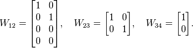
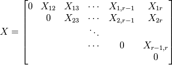
The following is an example of a basic Weyr matrix.

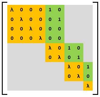
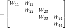
In this matrix,  and
and  . So has the Weyr structure
  . Also,
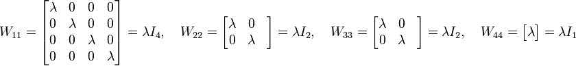
and
General Weyr matrix
Definition
Let be a square matrix and let  be the distinct eigenvalues of . We say that is in Weyr form (or is a Weyr matrix) if has the following form:
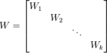
where  is a basic Weyr matrix with eigenvalue
  for
for  .
.
Example
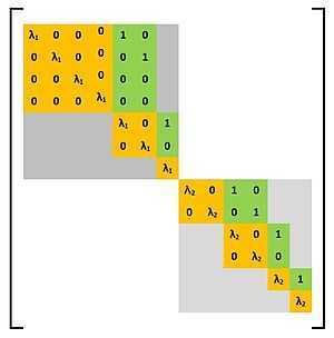
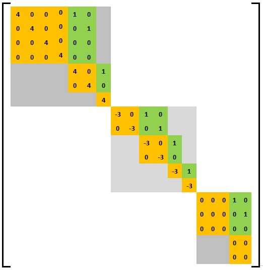
The following image shows an example of a general Weyr matrix consisting of three basic Weyr matrix blocks. The basic Weyr matrix in the top-left corner has the structure (4,2,1) with eigenvalue 4, the middle block has structure (2,2,1,1) with eigenvalue -3 and the one in the lower-right corner has the structure (3, 2) with eigenvalue 0.
The Weyr form is canonical
That the weyr form is a canonical form of a matrix is a consequence of the following result:[3] To within permutation of basic Weyr blocks, each square matrix  over an algebraically closed field is similar to a unique Weyr matrix . The matrix is called the Weyr (canonical ) form of .
Computation of the Weyr canonical form
Reduction to the nilpotent case
Let be a square matrix of order over an algebraically closed field and let the distinct eigenvalues of be 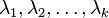 . As a consequence of the generalized eigenspace decomposition theorem, one can show that is similar to a block diagonal matrix of the form
where  is a diagonal matrix and
  is a nilpotent matrix. So the problem of reducing to the Weyr form reduces to the problem of reducing the nilpotent matrices
  to the Weyr form.
Reduction of a nilpotent matrix to the Weyr form
Given a nilpotent square matrix of order over an algebraically closed field  , the following algorithm produces an invertible matrix
  and a Weyr matrix such that
  .
.
Step 1
Let 
Step 2
- Compute a basis for the null space of
 .
. - Extend the basis for the null space of to a basis for the -dimensional vector space
 .
. - Form the matrix
 consisting of these basis vectors.
 - Compute
 .
.  is a square matrix of size − nullity
  .
.
Step 3
If is nonzero, repeat Step 2 on .
- Compute a basis for the null space of .
- Extend the basis for the null space of to a basis for the vector space having dimension − nullity .
- Form the matrix
 consisting of these basis vectors.
 - Compute
 . is a square matrix of size − nullity − nullity
 .
.
Step 4
Continue the processes of Steps 1 and 2 to obtain increasingly smaller square matrices  and associated nvertible matrices
  until the first zero matrix
  is obtained.
Step 5
The Weyr structure of is where  = nullity
 .
.
Step 6
- Compute the matrix
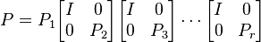 (here the
  's are appropriately sized identity matrices).
 - Compute
 .
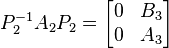
.  is a matrix of the following form:
-
 .
.
-
Step 7
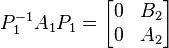
Use elementary row operations to find an invertible matrix  of appropriate size such that the product
  is a matrix of the form
 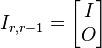 .
.
Step 8
Set  diag
diag 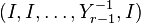 and compute
  . In this matrix, the
  -block is
  .
.
Step 9
Find a matrix  formed as a product of elementary matrices such that
 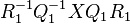 is a matrix in which all the blocks above the block contain only
  's.
's.
Step 10
Repeat Steps 8 and 9 on column  converting
  -block to
  via conjugation by some invertible matrix
  . Use this block to clear out the blocks above, via conjugation by a product
  of elementary matrices.
Step 11
Repeat these processes on  columns, using conjugations by
  . The resulting matrix is now in Weyr form.
Step 12
Let  . Then .
Applications of the Weyr form
Some well-known applications of the Weyr form are listed below:[3]
- The Weyr form can be used to simplify the proof of Gerstenhaber’s Theorem which asserts that the subalgebra generated by two commuting matrices has dimension at most .
- A set of finite matrices is said to be approximately simultaneously diagonalizable if they can be perturbed to simultaneously diagonalizable matrices. The Weyr form is used to prove approximate simultaneous diagonalizability of various classes of matrices. The approximate simultaneous diagonalizability property has applications in the study of phylogenetic invariants in biomathematics.
- The Weyr form can be used to simplify the proofs of the irreducibility of the variety of all k-tuples of commuting complex matrices.
References
- ↑ Eduard Weyr (1985). "Répartition des matrices en espèces et formation de toutes les espèces". Comptes Rendus, Paris 100: 966–969. Retrieved 10 December 2013.
- ↑ Eduard Weyr (1890). "Zur Theorie der bilinearen Formen". Monatsh. Math. Physik 1: 163–236.
- ↑ 3.0 3.1 3.2 3.3 Kevin C. Meara, John Clark, Charles I. Vinsonhaler (2011). Advanced Topics in Linear Algebra: Weaving Matrix Problems through the Weyr Form. Oxford University Press.
- ↑ 4.0 4.1 4.2 Kevin C. Meara, John Clark, Charles I. Vinsonhaler (2011). Advanced Topics in Linear Algebra: Weaving Matrix Problems through the Weyr Form. Oxford University Press. pp. 44, 81–82.
- ↑ Shapiro, H. (1999). "The Weyr characteristic". The American Mathematical Monthly 106: 919–929. doi:10.2307/2589746.