Weak formulation
Weak formulations are an important tool for the analysis of mathematical equations that permit the transfer of concepts of linear algebra to solve problems in other fields such as partial differential equations. In a weak formulation, an equation is no longer required to hold absolutely (and this is not even well defined) and has instead weak solutions only with respect to certain "test vectors" or "test functions". This is equivalent to formulating the problem to require a solution in the sense of a distribution.
We introduce weak formulations by a few examples and present the main theorem for the solution, the Lax–Milgram theorem.
General concept
Let  be a Banach space. We want to find the solution
  of the equation
 ,
,
where  and
and  , with
  being the dual of .
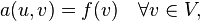
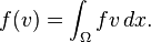
Calculus of variations tells us that this is equivalent to finding such that
for all  holds:
 = f(v)](../I/m/b39c30413b883a2dc617b92c2fc8d1a9.png) .
.
Here, we call  a test vector or test function.
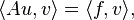
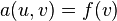
We bring this into the generic form of a weak formulation, namely, find such that
by defining the bilinear form
.](../I/m/90622c7d4ef9e6b813e2da7a36792241.png)
Since this is very abstract, let us follow this by some examples.
Example 1: linear system of equations
Now, let  and
and  a linear mapping. Then, the weak formulation of the equation
involves finding such that for all the following equation holds:
where  denotes an inner product.
Since  is a linear mapping, it is sufficient to test with basis vectors, and we get

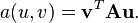
Actually, expanding  , we obtain the matrix form of the equation

where 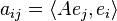 and
and  .
.
The bilinear form associated to this weak formulation is
Example 2: Poisson's equation
Our aim is to solve Poisson's equation

on a domain  with
with  on its boundary,
and we want to specify the solution space later. We will use the
on its boundary,
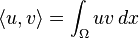
and we want to specify the solution space later. We will use the  -scalar product
to derive our weak formulation. Then, testing with differentiable functions , we get
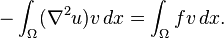
We can make the left side of this equation more symmetric by integration by parts using Green's identity:
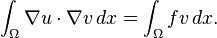
This is what is usually called the weak formulation of Poisson's equation; what's missing is the space , which is beyond the scope of this article. The space must allow us to write down this equation. Therefore, we should require that the derivatives of functions in this space are square integrable. Now, there is actually the Sobolev space  of functions with weak derivatives in
  and with zero boundary conditions, which fulfills this purpose.
We obtain the generic form by assigning
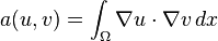
and
The Lax–Milgram theorem
This is a formulation of the Lax–Milgram theorem which relies on properties of the symmetric part of the bilinear form. It is not the most general form.
Let be a Hilbert space and  a bilinear form on , which is
 and
and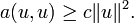
Then, for any , there is a unique solution to the equation
and it holds
Application to example 1
Here, application of the Lax–Milgram theorem is definitely overkill, but we still can use it and give this problem the same structure as the others have.
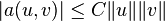
- Boundedness: all bilinear forms on
 are bounded. In particular, we have
- Coercivity: this actually means that the real parts of the eigenvalues of are not smaller than
 . Since this implies in particular that no eigenvalue is zero, the system is solvable.
Additionally, we get the estimate
where is the minimal real part of an eigenvalue of .
Application to example 2
Here, as we mentioned above, we choose  with the norm
where the norm on the right is the -norm on  (this provides a true norm on by the Poincaré inequality).
But, we see that
(this provides a true norm on by the Poincaré inequality).
But, we see that  and by the Cauchy–Schwarz inequality,
  .
.
Therefore, for any ![f\in [H^1_0(\Omega)]'](../I/m/ece1e2e27be8f721b7f66e3d48010e8e.png) , there is a unique solution of Poisson's equation and we have the estimate
, there is a unique solution of Poisson's equation and we have the estimate
![\|\nabla u\| \le \|f\|_{[H^1_0(\Omega)]'}.](../I/m/aea7250713d87831c3f2850f7fdc113a.png)
See also
References
- Lax, Peter D.; Milgram, Arthur N. (1954). "Parabolic equations". Contributions to the theory of partial differential equations. Annals of Mathematics Studies, no. 33. Princeton, N. J.: Princeton University Press. pp. 167–190. MR 0067317