Viola–Jones object detection framework
The Viola–Jones object detection framework is the first object detection framework to provide competitive object detection rates in real-time proposed in 2001 by Paul Viola and Michael Jones.[1][2] Although it can be trained to detect a variety of object classes, it was motivated primarily by the problem of face detection. This algorithm is implemented in OpenCV as cvHaarDetectObjects().
Problem description
The basic problem to be solved is to implement an algorithm for detection of faces in an image. This can be solved easily by humans. However there is a stark contrast to how difficult it actually is to make a computer successfully solve this task. In order to ease the task Viola–Jones limit themselves to full view frontal upright faces. That is, in order to be detected the entire face must point towards the camera and it should not be tilted to any side. This may compromise the requirement for being unconstrained a little bit, but considering that the detection algorithm most often will be succeeded by a recognition algorithm these demands seem quite reasonable.
Components of the framework

Feature types and evaluation
The main characteristics of Viola–Jones algorithm which makes it a good detection algorithm are:
- Robust – very high detection rate (true-positive rate) & very low false-positive rate always.
- Real time – For practical applications at least 2 frames per second must be processed.
- Face detection and not recognition - The goal is to distinguish faces from non-faces (face detection is the first step in the identification process)
The algorithm has mainly 4 stages:
- Haar Features Selection
- Creating Integral Image
- Adaboost Training algorithm
- Cascaded Classifiers
The features employed by the detection framework universally involve the sums of image pixels within rectangular areas. As such, they bear some resemblance to Haar basis functions, which have been used previously in the realm of image-based object detection.[3] However, since the features used by Viola and Jones all rely on more than one rectangular area, they are generally more complex. The figure at right illustrates the four different types of features used in the framework. The value of any given feature is always simply the sum of the pixels within clear rectangles subtracted from the sum of the pixels within shaded rectangles. As is to be expected, rectangular features of this sort are rather primitive when compared to alternatives such as steerable filters. Although they are sensitive to vertical and horizontal features, their feedback is considerably coarser.


1. Haar Features – All human faces share some similar properties. This knowledge is used to construct certain features known as Haar Features.
The properties that are similar for a human face are:
- The eyes region is darker than the upper-cheeks.
- The nose bridge region is brighter than the eyes.
That is useful domain knowledge:
- Location - Size: eyes & nose bridge region
- Value: darker / brighter
The four features applied in this algorithm are applied onto a face and shown on the left.
Rectangle features:
- Value = Σ (pixels in black area) - Σ (pixels in white area)
- Three types: two-, three-, four-rectangles, Viola & Jones used two-rectangle features
- For example: the difference in brightness between the white &black rectangles over a specific area
- Each feature is related to a special location in the sub-window
However, with the use of an image representation called the integral image, rectangular features can be evaluated in constant time, which gives them a considerable speed advantage over their more sophisticated relatives. Because each rectangular area in a feature is always adjacent to at least one other rectangle, it follows that any two-rectangle feature can be computed in six array references, any three-rectangle feature in eight,and any four-rectangle feature in just ten.
The integral image at location (x,y), is the sum of the pixels above and to the left of (x,y), inclusive.
Learning algorithm
The speed with which features may be evaluated does not adequately compensate for their number, however. For example, in a standard 24x24 pixel sub-window, there are a total of  [4] possible features, and it would be prohibitively expensive to evaluate them all when testing an image. Thus, the object detection framework employs a variant of the learning algorithm AdaBoost to both select the best features and to train classifiers that use them. This algorithm constructs a “strong” classifier as a linear combination of weighted simple “weak” classifiers.
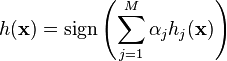
Each weak classifier is a threshold function based on the feature  .
.
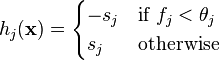
The threshold value  and the polarity
  are determine in the training, as well as the coefficients
  .
.
Here a simplified version of the learning algorithm is reported:[5]
Input: Set of  positive and negative training images with their labels
  . If image
  is a face
  , if not
  .
.
- Initialization: assign a weight
 to each image .
 - For each feature with

- Renormalize the weights such that they sum to one.
- Apply the feature to each image in the training set, then find the optimal threshold and polarity
 that minimizes the weighted classification error. That is
 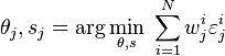 where
where 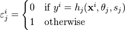
- Assign a weight to
 that is inversely proportional to the error rate. In this way best classifiers are considered more.
 - The weights for the next iteration, i.e.
 , are reduced for the images that were correctly classified.
- Set the final classifier to
Cascade architecture
- On average only 0.01% of all sub-windows are positive (faces)
- Equal computation time is spent on all sub-windows
- Must spend most time only on potentially positive sub-windows.
- A simple 2-feature classifier can achieve almost 100% detection rate with 50% FP rate.
- That classifier can act as a 1st layer of a series to filter out most negative windows
- 2nd layer with 10 features can tackle “harder” negative-windows which survived the 1st layer, and so on…
- A cascade of gradually more complex classifiers achieves even better detection rates.The evaluation of the strong classifiers generated by the learning process can be done quickly, but it isn’t fast enough to run in real-time. For this reason, the strong classifiers are arranged in a cascade in order of complexity, where each successive classifier is trained only on those selected samples which pass through the preceding classifiers. If at any stage in the cascade a classifier rejects the sub-window under inspection, no further processing is performed and continue on searching the next sub-window (see figure at right). The cascade therefore has the form of a degenerate tree. In the case of faces, the first classifier in the cascade – called the attentional operator – uses only two features to achieve a false negative rate of approximately 0% and a false positive rate of 40%.[6] The effect of this single classifier is to reduce by roughly half the number of times the entire cascade is evaluated.
In cascading, each stage consists of a strong classifier. So all the features are grouped into several stages where each stage has certain number of features.
The job of each stage is to determine whether a given sub-window is definitely not a face or may be a face. A given sub-window is immediately discarded as not a face if it fails in any of the stages.
A simple framework for cascade training is given below:
- User selects values for f, the maximum acceptable false positive rate per layer and d, the minimum acceptable detection rate per layer.
- User selects target overall false positive rate Ftarget.
- P = set of positive examples
- N = set of negative examples
- F(0) = 1.0; D(0) = 1.0; i = 0
 while F(i) > Ftarget
     i++
     n(i) = 0; F(i)= F(i-1)

     while F(I) > f x F(i-1)
      - n(i) ++
      - use P and N to train a classifier with n(I) features using AdaBoost
      - Evaluate current cascaded classifier on validation set to determine F(i) & D(i)
      - decrease threshold for the ith classifier until the current cascaded classifier has a detection rate of at least d x D(i-1) (this also affects F(i))
      - N = ∅
      - If F(i) > Ftarget then evaluate the current cascaded detector on the set of non-face images and put any false detections into the set N.
The cascade architecture has interesting implications for the performance of the individual classifiers. Because the activation of each classifier depends entirely on the behavior of its predecessor, the false positive rate for an entire cascade is:

Similarly, the detection rate is:

Thus, to match the false positive rates typically achieved by other detectors, each classifier can get away with having surprisingly poor performance. For example, for a 32-stage cascade to achieve a false positive rate of  , each classifier need only achieve a false positive rate of about 65%. At the same time, however, each classifier needs to be exceptionally capable if it is to achieve adequate detection rates. For example, to achieve a detection rate of about 90%, each classifier in the aforementioned cascade needs to achieve a detection rate of approximately 99.7%.
Advantages of Viola–Jones algorithm
- Extremely fast feature computation
- Efficient feature selection
- Scale and location invariant detector
- Instead of scaling the image itself (e.g. pyramid-filters), we scale the features.
- Such a generic detection scheme can be trained for detection of other types of objects (e.g. cars, hands)
Disadvantages of Viola–Jones algorithm
- Detector is most effective only on frontal images of faces
- It can hardly cope with 45° face rotation both around the vertical and horizontal axis.
- Sensitive to lighting conditions
- We might get multiple detections of the same face, due to overlapping sub-windows.

MATLAB code for using the cascadeObjectDetector() function
clear all
vid = videoinput('winvideo', 1, 'YUY2_640x480'); % Giving the framesize
vid.ReturnedColorSpace = 'RGB'; % Mentioning RGB format
vid.TriggerRepeat = Inf; % Triggers the camera repeatedly
vid.FrameGrabInterval = 1; % Time between successive frames
start(vid); % Starts capturing video
detector = vision.CascadeObjectDetector(); % Create a detector using Viola-Jones
while true % Infinite loop to continuously detect the face
    img = flipdim(getdata(vid, 1), 2); % Flips the image horizontally
    imshow(img); hold on; % Displays image
    bbox = step(detector, img); % Creating bounding box using detector
    if ~ isempty(bbox)
        rectangle('position', bbox(1, :), 'lineWidth', 2, 'edgeColor', 'y');
    end % Draws a yellow rectangle around the detected face
    flushdata(vid);
    hold off;
end
Related face detection and tracking algorithm
The algorithm that is similar to Viola–Jones but can detect and track even tilted and rotated faces is the KLT algorithm. Here the feature points are detected by scanning the face initially. Thereafter, the face can be detected and tracked even when the face is tilted and further away from the camera, which is not possible in case of Viola–Jones algorithm.[7]
Improvements over the Viola–Jones algorithm
An improved algorithm on Viola–Jones object detector[8]
MATLAB implementation of Viola–Jones algorithm[9]
OpenCV implementation of Viola–Jones algorithm
Haar Cascade Detection in OpenCV[10]
Cascade Classifier Training in OpenCV[11]
Citations of the Viola–Jones algorithm in Google Scholar[12]
Implementing the Viola–Jones Face Detection Algorithm by Ole Helvig Jensen[13]
Adaboost Explanation from ppt by Qing Chen, Discovery Labs, University of Ottawa and a video lecture by Ramsri Goutham.
Video link - [14]
References
- ↑ Rapid object detection using a boosted cascade of simple features
- ↑ Viola, Jones: Robust Real-time Object Detection, IJCV 2001 See pages 1,3.
- ↑ C. Papageorgiou, M. Oren and T. Poggio. A General Framework for Object Detection. International Conference on Computer Vision, 1998
- ↑ Viola-Jones’ face detection claims 180k features
- ↑ R. Szeliski, Computer Vision, algorithms and applications, Springer
- ↑ Viola, Jones: Robust Real-time Object Detection, IJCV 2001 See page 11.
- ↑ Face Detection and Tracking using the KLT algorithm
- ↑ Improved algorithm than Viola–Jones
- ↑ MATLAB implementation of Viola–Jones algorithm
- ↑ OpenCV Implementation of Viola–Jones
- ↑ Cascade Classifier Training in OpenCV
- ↑ Citations of the Viola–Jones algorithm in Google Scholar
- ↑ Implementing Viola–Jones
- ↑ Video lecture on Viola–Jones algorithm
External links
- MATLAB implementation Viola–Jones detection
- Slides Presenting the Framework
- Information Regarding Haar Basis Functions
- Extension of Viola–Jones framework using SURF feature
- IMMI - Rapidminer Image Mining Extension - open-source tool for image mining
- Wikipedia:WikiProject Computer Vision
- Robust Real-Time Face Detection