Variogram

In spatial statistics the theoretical variogram $2\gamma(x,y)$ is a function describing the degree of spatial dependence of a spatial random field or stochastic process $Z(x)$ . It is defined as the variance of the difference between field values at two locations ( $x$ and $y$ ) across realizations of the field (Cressie 1993):

2\gamma(x,y)=\text{var}\left(Z(x) - Z(y)\right) = E\left[((Z(x)-\mu(x))-(Z(y) - \mu(y)))^2\right].

If the spatial random field has constant mean $\mu$ , this is equivalent to the expectation for the squared increment of the values between locations $x$ and $y$ (Wackernagel 2003) (where $x$ and $y$ are not coordinates but points in space):

2\gamma(x,y)=E\left[\left(Z(x)-Z(y)\right)^2\right] ,

where $\gamma(x,y)$ itself is called the semivariogram. In the case of a stationary process, the variogram and semivariogram can be represented as a function $\gamma_s(h)=\gamma(0,0+h)$ of the difference $h=y-x$ between locations only, by the following relation (Cressie 1993):

\gamma(x,y)=\gamma_s(y-x).

If the process is furthermore isotropic, then the variogram and semivariogram can be represented by a function $\gamma_i(h):=\gamma_s(h e_1)$ of the distance $h=\|y-x\|$ only (Cressie 1993):

\gamma(x,y)=\gamma_i(h).

The indexes $i$ or $s$ are typically not written. The terms are used for all three forms of the function. Moreover, the term "variogram" is sometimes used to denote the semivariogram, and the symbol $\gamma$ is sometimes used for the variogram, which brings some confusion.

Properties

According to (Cressie 1993, Chiles and Delfiner 1999, Wackernagel 2003) the theoretical variogram has the following properties:

The semivariogram is nonnegative $\gamma(x,y)\geq 0$ , since it is the expectation of a square.
The semivariogram $\gamma(x,x)=\gamma_i(0)=E\left((Z(x)-Z(x))^2\right)=0$ at distance 0 is always 0, since $Z(x)-Z(x)=0$ .
A function is a semivariogram if and only if it is a conditionally negative definite function, i.e. for all weights $w_1,\ldots,w_N$ subject to $\sum_{i=1}^N w_i=0$ and locations $x_1,\ldots,x_N$ it holds:
$\sum_{i=1}^N\sum_{j=1}^N w_{i}\gamma(x_i,x_j)w_j \leq 0$
which corresponds to the fact that the variance $var(X)$ of $X=\sum_{i=1}^N w_i Z(x_i)$ is given by the negative of this double sum and must be nonnegative.
As a consequence the semivariogram might be non continuous only at the origin. The height of the jump at the origin is sometimes referred to as nugget or nugget effect.
If the covariance function of a stationary process exists it is related to variogram by
$2\gamma(x,y)=C(x,x)+C(y,y)-2C(x,y)$
For a non-stationary process the square of the difference between expected values at both points must be added:
$2\gamma(x,y)=C(x,x)+C(y,y)-2C(x,y) + (E\left[Z(x)\right]-E\left[Z(y)\right])^2$
If a stationary random field has no spatial dependence (i.e. $C(h)=0$ if $h\not= 0$ ), the semivariogram is the constant $var(Z(x))$ everywhere except at the origin, where it is zero.
$\gamma(x,y)=E\left[|Z(x)-Z(y)|^2\right]=\gamma(y,x)$ is a symmetric function.
Consequently, $\gamma_s(h)=\gamma_s(-h)$ is an even function.
If the random field is stationary and ergodic, the $\lim_{h\to \infty} \gamma_s(h) = var(Z(x))$ corresponds to the variance of the field. The limit of the semivariogram is also called its sill.

Empirical variogram

For observations $z_i,\;i=1,\ldots,k$ at locations $x_1,\ldots,x_k$ the empirical variogram $\hat{\gamma}(h)$ is defined as (Cressie 1993):

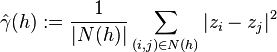
$\hat{\gamma}(h):=\frac{1}{|N(h)|}\sum_{(i,j)\in N(h)} |z_i-z_j|^2$

where $N(h)$ denotes the set of pairs of observations $i,\;j$ such that $|x_i-x_j| = h$ , and $|N(h)|$ is the number of pairs in the set. (Generally an "approximate distance" $h$ is used, implemented using a certain tolerance.)

The empirical variogram is used in geostatistics as a first estimate of the (theoretical) variogram needed for spatial interpolation by kriging.

According to (Cressie 1993), for observations $z_i=Z(x_i)$ from a stationary random field $Z(x)$ , the empirical variogram with lag tolerance 0 is an unbiased estimator of the theoretical variogram, due to:

$E\left[\hat{\gamma}(h)\right]=\frac{1}{2|N(h)|}\sum_{(i,j)\in N(h)}E\left[|Z(x_i)-Z(x_j)|^2\right]=\frac{1}{2|N(h)|}\sum_{(i,j)\in N(h)}2\gamma(x_j-x_i)=\frac{2|N(h)|}{2|N(h)|}\gamma(h)$

Variogram parameters

The following parameters are often used to describe variograms:

nugget $n$ : The height of the jump of the semivariogram at the discontinuity at the origin.
sill $s$ : Limit of the variogram tending to infinity lag distances.
range $r$ : The distance in which the difference of the variogram from the sill becomes negligible. In models with a fixed sill, it is the distance at which this is first reached; for models with an asymptotic sill, it is conventionally taken to be the distance when the semivariance first reaches 95% of the sill.

Variogram models

The empirical variogram cannot be computed at every lag distance $h$ and due to variation in the estimation it is not ensured that it is a valid variogram, as defined above. However some Geostatistical methods such as kriging need valid semivariograms. In applied geostatistics the empirical variograms are thus often approximated by model function ensuring validity (Chiles&Delfiner 1999). Some important models are (Chiles&Delfiner 1999, Cressie 1993):

The exponential variogram model

\gamma(h)=(s-n)(1-\exp(-h/(ra)))+n 1_{(0,\infty)}(h)

The spherical variogram model

\gamma(h)=(s-n)\left(\left(\frac{3h}{2r}-\frac{h^3}{2r^3}\right)1_{(0,r)}(h)+1_{[r,\infty)}(h)\right)+n1_{(0,\infty)}(h)

The Gaussian variogram model

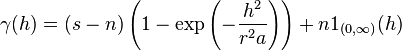
\gamma(h)=(s-n)\left(1-\exp\left(-\frac{h^2}{r^2a}\right)\right) + n1_{(0,\infty)}(h)

The parameter $a$ has different values in different references, due to the ambiguity in the definition of the range. E.g. $a=1/3$ is the value used in (Chiles&Delfiner 1999). The $1_A(h)$ function is 1 if $h\in A$ and 0 otherwise.

Discussion

Three functions are used in geostatistics for describing the spatial or the temporal correlation of observations: these are the correlogram, the covariance and the semivariogram. The last is also more simply called variogram. The sampling variogram, unlike the semivariogram and the variogram, shows where a significant degree of spatial dependence in the sample space or sampling unit dissipates into randomness when the variance terms of a temporally or in-situ ordered set are plotted against the variance of the set and the lower limits of its 99% and 95% confidence ranges.

The variogram is the key function in geostatistics as it will be used to fit a model of the temporal/spatial correlation of the observed phenomenon. One is thus making a distinction between the experimental variogram that is a visualisation of a possible spatial/temporal correlation and the variogram model that is further used to define the weights of the kriging function. Note that the experimental variogram is an empirical estimate of the covariance of a Gaussian process. As such, it may not be positive definite and hence not directly usable in kriging, without constraints or further processing. This explains why only a limited number of variogram models are used: most commonly, the linear, the spherical, the gaussian and the exponential models.

When a variogram is used to describe the correlation of different variables it is called cross-variogram. Cross-variograms are used in co-kriging. Should the variable be binary or represent classes of values, one is then talking about indicator variograms. Indicator variogram is used in indicator kriging.

References

Cressie, N., 1993, Statistics for spatial data, Wiley Interscience
Chiles, J. P., P. Delfiner, 1999, Geostatististics, Modelling Spatial Uncertainty, Wiley-Interscience
Wackernagel, H., 2003, Multivariate Geostatistics, Springer
Burrough, P A and McDonnell, R A, 1998, Principles of Geographical Information Systems
Isobel Clark, 1979, Practical Geostatistics, Applied Science Publishers