Uncertainty theory
Uncertainty theory is a branch of mathematics based on normality, monotonicity, self-duality, countable subadditivity, and product measure axioms. It was founded by Baoding Liu [1] in 2007 and refined in 2009.[2]
Mathematical measures of the likelihood of an event being true include probability theory, capacity, fuzzy logic, possibility, and credibility, as well as uncertainty.
Five axioms
Axiom 1. (Normality Axiom)  .
.
Axiom 2. (Monotonicity Axiom)  .
.
Axiom 3. (Self-Duality Axiom)  .
.
Axiom 4. (Countable Subadditivity Axiom) For every countable sequence of events Λ1, Λ2, ..., we have
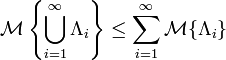 .
.
Axiom 5. (Product Measure Axiom) Let  be uncertainty spaces for
  . Then the product uncertain measure
  is an uncertain measure on the product σ-algebra satisfying
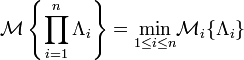 .
.
Principle. (Maximum Uncertainty Principle) For any event, if there are multiple reasonable values that an uncertain measure may take, then the value as close to 0.5 as possible is assigned to the event.
Uncertain variables
An uncertain variable is a measurable function ξ from an uncertainty space  to the set of real numbers, i.e., for any Borel set B of real numbers, the set
 is an event.
Uncertainty distribution
Uncertainty distribution is inducted to describe uncertain variables.
Definition:The uncertainty distribution ![\Phi(x):R \rightarrow [0,1]](../I/m/111a66c8ad3deba6e3e930ac8981f090.png) of an uncertain variable ξ is defined by
of an uncertain variable ξ is defined by  .
.
Theorem(Peng and Iwamura, Sufficient and Necessary Condition for Uncertainty Distribution) A function is an uncertain distribution if and only if it is an increasing function except  and
and  .
.
Independence
Definition: The uncertain variables  are said to be independent if

for any Borel sets  of real numbers.
Theorem 1: The uncertain variables are independent if

for any Borel sets of real numbers.
Theorem 2: Let be independent uncertain variables, and  measurable functions. Then
 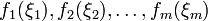 are independent uncertain variables.
Theorem 3: Let  be uncertainty distributions of independent uncertain variables
  respectively, and
  the joint uncertainty distribution of uncertain vector
  . If are independent, then we have

for any real numbers  .
.
Operational law
Theorem: Let be independent uncertain variables, and  a measurable function. Then
  is an uncertain variable such that
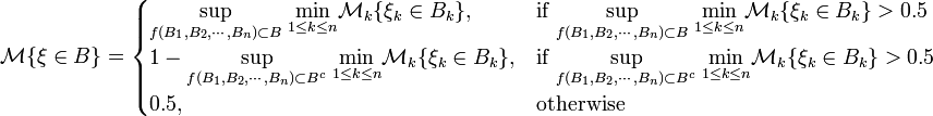
where  are Borel sets, and
  means
means for any
 .
.
Expected Value
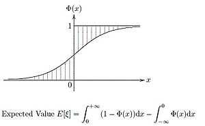
Definition: Let  be an uncertain variable. Then the expected value of is defined by
![E[\xi]=\int_0^{+\infty}M\{\xi\geq r\}dr-\int_{-\infty}^0M\{\xi\leq r\}dr](../I/m/4acefaa4ff23e180c09b33f108cd9d48.png)
provided that at least one of the two integrals is finite.
Theorem 1: Let be an uncertain variable with uncertainty distribution . If the expected value exists, then
![E[\xi]=\int_0^{+\infty}(1-\Phi(x))dx-\int_{-\infty}^0\Phi(x)dx](../I/m/4ad88bdee5187c99bc96c9ad339ed932.png) .
.
Theorem 2: Let be an uncertain variable with regular uncertainty distribution . If the expected value exists, then
![E[\xi]=\int_0^1\Phi^{-1}(\alpha)d\alpha](../I/m/c582acb4d985e5f838a9c3fcae7a6cdb.png) .
.
Theorem 3: Let and  be independent uncertain variables with finite expected values. Then for any real numbers
  and
and  , we have
![E[a\xi+b\eta]=aE[\xi]+b[\eta]](../I/m/1bd1996a9c074c5b644482d544b31ca5.png) .
.
Variance
Definition: Let be an uncertain variable with finite expected value  . Then the variance of is defined by
![V[\xi]=E[(\xi-e)^2]](../I/m/1746eb406f832334f9ebdac4906ce839.png) .
.
Theorem: If be an uncertain variable with finite expected value, and are real numbers, then
![V[a\xi+b]=a^2V[\xi]](../I/m/58560bbfbb2912baf08d3d14492a7ccd.png) .
.
Critical value
Definition: Let be an uncertain variable, and ![\alpha\in(0,1]](../I/m/a20ad44a15374ffd41728fbd75899830.png) . Then
. Then

is called the α-optimistic value to , and

is called the α-pessimistic value to .
Theorem 1: Let be an uncertain variable with regular uncertainty distribution . Then its α-optimistic value and α-pessimistic value are
 ,
, .
.
Theorem 2: Let be an uncertain variable, and . Then we have
- if
 , then
  ;
; - if
 , then
  .
.
Theorem 3: Suppose that and are independent uncertain variables, and . Then we have
 ,
,
 ,
,
 ,
,
 ,
,
 ,
,
 .
.
Entropy
Definition: Let be an uncertain variable with uncertainty distribution . Then its entropy is defined by
![H[\xi]=\int_{-\infty}^{+\infty}S(\Phi(x))dx](../I/m/baf65dcc46ef68511a6cf25e174bae58.png)
where  .
.
Theorem 1(Dai and Chen): Let be an uncertain variable with regular uncertainty distribution . Then
![H[\xi]=\int_0^1\Phi^{-1}(\alpha)\mbox{ln}\frac{\alpha}{1-\alpha}d\alpha](../I/m/49c978309a96c03da01cf99bfa5e16fd.png) .
.
Theorem 2: Let and be independent uncertain variables. Then for any real numbers and , we have
![H[a\xi+b\eta]=|a|E[\xi]+|b|E[\eta]](../I/m/c8d323c30b0ba0d1507867c412c504c0.png) .
.
Theorem 3: Let be an uncertain variable whose uncertainty distribution is arbitrary but the expected value and variance  . Then
![H[\xi]\leq\frac{\pi\sigma}{\sqrt{3}}](../I/m/7dc0d8cd666800255eac3f2913993f2d.png) .
.
Inequalities
Theorem 1(Liu, Markov Inequality): Let be an uncertain variable. Then for any given numbers  and
and  , we have
![M\{|\xi|\geq t\}\leq \frac{E[|\xi|^p]}{t^p}](../I/m/e046a131a3843627ba0a826cbb2ffa8e.png) .
.
Theorem 2 (Liu, Chebyshev Inequality) Let be an uncertain variable whose variance ![V[\xi]](../I/m/8232e3d17f1eea4e9a4a0770f81e9330.png) exists. Then for any given number, we have
exists. Then for any given number, we have
![M\{|\xi-E[\xi]|\geq t\}\leq \frac{V[\xi]}{t^2}](../I/m/de850f0f17d65b26aa6a56dcd6bbcf88.png) .
.
Theorem 3 (Liu, Holder’s Inequality) Let  and
and  be positive numbers with
  , and let and be independent uncertain variables with
 ![E[|\xi|^p]< \infty](../I/m/11487b46691f80fc5900338f5e73a342.png) and
and ![E[|\eta|^q] < \infty](../I/m/7c8a36cacc1c7fdfc54afb97c9b1a068.png) . Then we have
. Then we have
![E[|\xi\eta|]\leq \sqrt[p]{E[|\xi|^p]} \sqrt[p]{E[\eta|^p]}](../I/m/2057ae295c705f7e28e47f51929ec50e.png) .
.
Theorem 4:(Liu [127], Minkowski Inequality) Let be a real number with  , and let and be independent uncertain variables with and . Then we have
![\sqrt[p]{E[|\xi+\eta|^p]}\leq \sqrt[p]{E[|\xi|^p]}+\sqrt[p]{E[\eta|^p]}](../I/m/849d1421275276e6151312cd73e0d5b6.png) .
.
Convergence concept
Definition 1: Suppose that  are uncertain variables defined on the uncertainty space . The sequence
  is said to be convergent a.s. to if there exists an event
  with
with  such that
for every  . In that case we write
  ,a.s.
,a.s.
Definition 2: Suppose that are uncertain variables. We say that the sequence converges in measure to if

for every  .
.
Definition 3: Suppose that are uncertain variables with finite expected values. We say that the sequence converges in mean to if
![\mbox{lim}_{i\rightarrow\infty}E[|\xi_i-\xi|]=0](../I/m/35869cc4f7fbd26c401b35a468e43d7a.png) .
.
Definition 4: Suppose that  are uncertainty distributions of uncertain variables , respectively. We say that the sequence converges in distribution to if
  at any continuity point of .
Theorem 1: Convergence in Mean  Convergence in Measure Convergence in Distribution.
However, Convergence in Mean
Convergence in Measure Convergence in Distribution.
However, Convergence in Mean  Convergence Almost Surely Convergence in Distribution.
Conditional uncertainty
Definition 1: Let be an uncertainty space, and  . Then the conditional uncertain measure of A given B is defined by

Theorem 1: Let be an uncertainty space, and B an event with  . Then M{·|B} defined by Definition 1 is an uncertain measure, and
  is an uncertainty space.
Definition 2: Let be an uncertain variable on . A conditional uncertain variable of given B is a measurable function  from the conditional uncertainty space
  to the set of real numbers such that
 .
.
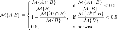
Definition 3: The conditional uncertainty distribution ![\Phi\rightarrow[0, 1]](../I/m/81b3150555bb3427d785cb630a338e66.png) of an uncertain variable given B is defined by
of an uncertain variable given B is defined by
provided that .
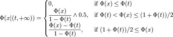
Theorem 2: Let be an uncertain variable with regular uncertainty distribution  , and
, and  a real number with
  . Then the conditional uncertainty distribution of given
  is
is
Theorem 3: Let be an uncertain variable with regular uncertainty distribution , and a real number with  . Then the conditional uncertainty distribution of given
  is
is
![\Phi(x\vert(-\infty,t])=\begin{cases} \displaystyle\frac{\Phi(x)}{\Phi(t)}, & \text{if }\Phi(x)\le\Phi(t)/2 \\ \displaystyle\frac{\Phi(x)+\Phi(t)-1}{\Phi(t)}\or 0.5, & \text{if }\Phi(t)/2\le\Phi(x)<\Phi(t) \\ 1, & \text{if }\Phi(t)\le\Phi(x) \end{cases}](../I/m/55030488f0a0dddea69dacd8a179a9bf.png)
Definition 4: Let be an uncertain variable. Then the conditional expected value of given B is defined by
![E[\xi|B]=\int_0^{+\infty}M\{\xi\geq r|B\}dr-\int_{-\infty}^0M\{\xi\leq r|B\}dr](../I/m/db46d421caea53e2498bd705e17bac63.png)
provided that at least one of the two integrals is finite.
References
- ↑ Baoding Liu, Uncertainty Theory, 2nd ed., Springer-Verlag, Berlin, 2007.
- ↑ Baoding Liu, Uncertainty Theory, 4th ed., http://orsc.edu.cn/liu/ut.pdf.
- Xin Gao, Some Properties of Continuous Uncertain Measure, International Journal of Uncertainty, Fuzziness and Knowledge-Based Systems, Vol.17, No.3, 419-426, 2009.
- Cuilian You, Some Convergence Theorems of Uncertain Sequences, Mathematical and Computer Modelling, Vol.49, Nos.3-4, 482-487, 2009.
- Yuhan Liu, How to Generate Uncertain Measures, Proceedings of Tenth National Youth Conference on Information and Management Sciences, August 3–7, 2008, Luoyang, pp. 23–26.
- Baoding Liu, Some Research Problems in Uncertainty Theory, Journal of Uncertain Systems, Vol.3, No.1, 3-10, 2009.
- Yang Zuo, Xiaoyu Ji, Theoretical Foundation of Uncertain Dominance, Proceedings of the Eighth International Conference on Information and Management Sciences, Kunming, China, July 20–28, 2009, pp. 827–832.
- Yuhan Liu and Minghu Ha, Expected Value of Function of Uncertain Variables, Proceedings of the Eighth International Conference on Information and Management Sciences, Kunming, China, July 20–28, 2009, pp. 779–781.
- Zhongfeng Qin, On Lognormal Uncertain Variable, Proceedings of the Eighth International Conference on Information and Management Sciences, Kunming, China, July 20–28, 2009, pp. 753–755.
- Jin Peng, Value at Risk and Tail Value at Risk in Uncertain Environment, Proceedings of the Eighth International Conference on Information and Management Sciences, Kunming, China, July 20–28, 2009, pp. 787–793.
- Yi Peng, U-Curve and U-Coefficient in Uncertain Environment, Proceedings of the Eighth International Conference on Information and Management Sciences, Kunming, China, July 20–28, 2009, pp. 815–820.
- Wei Liu, Jiuping Xu, Some Properties on Expected Value Operator for Uncertain Variables, Proceedings of the Eighth International Conference on Information and Management Sciences, Kunming, China, July 20–28, 2009, pp. 808–811.
- Xiaohu Yang, Moments and Tails Inequality within the Framework of Uncertainty Theory, Proceedings of the Eighth International Conference on Information and Management Sciences, Kunming, China, July 20–28, 2009, pp. 812–814.
- Yuan Gao, Analysis of k-out-of-n System with Uncertain Lifetimes, Proceedings of the Eighth International Conference on Information and Management Sciences, Kunming, China, July 20–28, 2009, pp. 794–797.
- Xin Gao, Shuzhen Sun, Variance Formula for Trapezoidal Uncertain Variables, Proceedings of the Eighth International Conference on Information and Management Sciences, Kunming, China, July 20–28, 2009, pp. 853–855.
- Zixiong Peng, A Sufficient and Necessary Condition of Product Uncertain Null Set, Proceedings of the Eighth International Conference on Information and Management Sciences, Kunming, China, July 20–28, 2009, pp. 798–801.