Trend stationary

In the statistical analysis of time series, a stochastic process is trend stationary if an underlying trend (function solely of time) can be removed, leaving a stationary process.^[1]

Formal definition

A process {Y} is said to be trend stationary if^[2]

Y_t = f(t) + e_t,

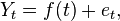
where t is time, f is any function mapping from the reals to the reals, and {e} is a stationary process. The value $f(t)$ is said to be the trend value of the process at time t.

Simplest example: stationarity around a linear trend

Suppose the variable Y evolves according to

Y_t = a \cdot t + b + e_t

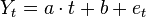
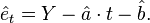
where t is time and e_t is the error term, which is hypothesized to be white noise or more generally to have been generated by any stationary process. Then one can use^[2]^[3]^[4]linear regression to obtain an estimate $\hat{a}$ of the true underlying trend slope $a$ and an estimate $\hat{b}$ of the underlying intercept term b; if the estimate $\hat{a}$ is significantly different from zero, this is sufficient to show with high confidence that the variable Y is non-stationary. The residuals from this regression are given by

\hat{e}_t = Y - \hat{a} \cdot t - \hat{b}.

If these estimated residuals can be statistically shown to be stationary (more precisely, if one can reject the hypothesis that the true underlying errors are non-stationary), then the residuals are referred to as the detrended data,^[5] and the original series {Y_t} is said to be trend stationary even though it is not stationary.

Stationarity around other types of trend

Exponential growth trend

Many economic time series are characterized by exponential growth. For example, suppose that one hypothesizes that gross domestic product is characterized by stationary deviations from a trend involving a constant growth rate. Then it could be modeled as

\text{GDP}_t = Be^{at}U_t

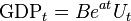
with U_t being hypothesized to be a stationary error process. To estimate the parameters $a$ and B, one first takes^[5] the natural logarithm (ln) of both sides of this equation:

\ln (\text{GDP}_t) = \ln B + at + \ln (U_t).

This log-linear equation is in the same form as the previous linear trend equation and can be detrended in the same way, giving the estimated $(\ln U)_t$ as the detrended value of $(\ln \text{GDP})_t$ , and hence the implied $U_t$ as the detrended value of $\text{GDP}_t$ , assuming one can reject the hypothesis that $(\ln U)_t$ is non-stationary.

Quadratic trend

Trends do not have to be linear or log-linear. For example, a variable could have a quadratic trend:

Y_t = a \cdot t + c \cdot t^2 + b + e_t.

This can be regressed linearly in the coefficients using t and t² as regressors; again, if the residuals are shown to be stationary then they are the detrended values of $Y_t$ .

Other non-stationary processes that are not trend stationary but can be rendered stationary

Trend stationary processes are not the only kind of non-stationary process that can be transformed into a stationary one; another prominent such process exhibits one or more unit roots^[2]^[3]^[4]^[5] but has all its other roots smaller than unity in magnitude.

Notes

↑ About.com economics Online Glossary of Research Economics
↑ 2.0 2.1 2.2 Nelson, Charles R. and Plosser, Charles I. (1982), "Trends and Random Walks in Macroeconomic Time Series: Some Evidence and Implications," Journal of Monetary Economics, 10, 139-162.
↑ 3.0 3.1 Hegwood, Natalie, and Papell,David H. "Are real GDP levels trend, difference, or regime-wise trend stationary? Evidence from panel data tests incorporating structural change." http://www.uh.edu/~dpapell/realgdp.pdf
↑ 4.0 4.1 Lucke, Bernd. "Is Germany‘s GDP trend-stationary? A measurement-with-theory approach." http://www.wiso.uni-hamburg.de/fileadmin/wiso_vwl_iwk/paper/gdptrend.pdf
↑ 5.0 5.1 5.2 http://www.duke.edu/~rnau/411diff.htm "Stationarity and differencing"