Transverse isotropy

A transversely isotropic material is one with physical properties which are symmetric about an axis that is normal to a plane of isotropy. This transverse plane has infinite planes of symmetry and thus, within this plane, the material properties are the same in all directions. Hence, such materials are also known as "polar anisotropic" materials.
This type of material exhibits hexagonal symmetry, so the number of independent constants in the (fourth-rank) elasticity tensor are reduced to 5 (from a total of 21 independent constants in the case of a fully anisotropic solid). The (second-rank) tensors of electrical resistivity, permeability, etc. have 2 independent constants.
Example of transversely isotropic materials
An example of a transversely isotropic material is the so-called on-axis unidirectional fiber composite lamina where the fibers are circular in cross section. In a unidirectional composite, the plane normal to the fiber direction can be considered as the isotropic plane, at long wavelengths (low frequencies) of excitation. In the figure to the right, the fibers would be aligned with the  axis, which is normal to the plane of isotropy.
In terms of effective properties, geological layers of rocks are often interpreted as being transversely isotropic. Calculating the effective elastic properties of such layers in petrology has been coined Backus upscaling, which is described below.
Material symmetry matrix
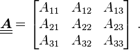
The material matrix  has a symmetry with respect to a given orthogonal transformation (
 ) if it does not change when subjected to that transformation.
For invariance of the material properties under such a transformation we require
) if it does not change when subjected to that transformation.
For invariance of the material properties under such a transformation we require

Hence the condition for material symmetry is (using the definition of an orthogonal transformation)

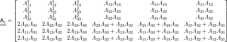
Orthogonal transformations can be represented in Cartesian coordinates by a  matrix
  given by
Therefore the symmetry condition can be written in matrix form as

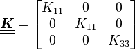
For a transversely isotropic material, the matrix has the form
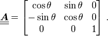
where the  -axis is the axis of symmetry. The material matrix remains invariant under rotation by any angle
  about the -axis.
Transverse isotropy in physics
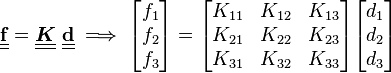
Linear material constitutive relations in physics can be expressed in the form

where  are two vectors representing physical quantities and
  is a second-order material tensor. In matrix form,
Examples of physical problems that fit the above template are listed in the table below [1]
| Problem |  |  | |
|---|---|---|---|
| Electrical conduction | Electrical current  | Electric field  | Electrical conductivity  |
| Dielectrics | Electrical displacement  | Electric field | Electric permittivity  |
| Magnetism | Magnetic induction  | Magnetic field  | Magnetic permeability  |
| Thermal conduction | Heat flux  | Temperature gradient  | Thermal conductivity  |
| Diffusion | Particle flux | Concentration gradient | Diffusivity |
| Flow in porous media | Weighted fluid velocity  | Pressure gradient  | Fluid permeability |
Using  in the matrix implies that
  . Using
  leads to
  and
and 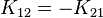 . Energy restrictions usually require
  and hence we must have
  . Therefore the material properties of a transversely isotropic material are described by the matrix
Transverse isotropy in linear elasticity
Condition for material symmetry
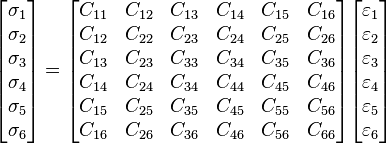
In linear elasticity, the stress and strain are related by Hooke's law, i.e.,

or, using Voigt notation,
The condition for material symmetry in linear elastic materials is.[2]
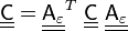
where
Elasticity tensor
Using the specific values of in matrix ,[3] it can be shown that the fourth-rank elasticity stiffness tensor may be written in 2-index Voigt notation as the matrix
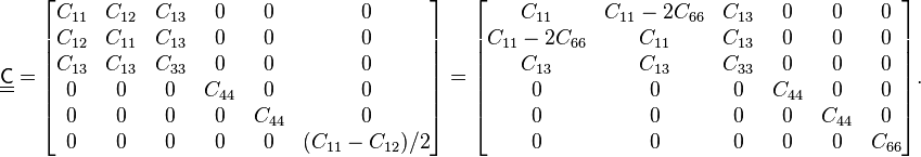
The elasticity stiffness matrix  has 5 independent constants, which are related to well known engineering elastic moduli in the following way. These engineering moduli are experimentally determined.
The compliance matrix (inverse of the elastic stiffness matrix) is
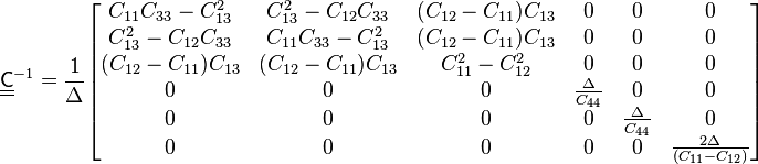
where ![\Delta := (C_{11} - C_{12}) [(C_{11} + C_{12}) C_{33} -2 C_{13}C_{13}]](../I/m/649b98b8652d8fb52684900b812a4927.png) . In engineering notation,
. In engineering notation,
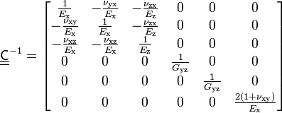
Comparing these two forms of the compliance matrix shows us that the longitudinal Young's modulus is given by

Similarly, the transverse Young's modulus is

The inplane shear modulus is

and the Poisson's ratio for loading along the polar axis is
 .
.
Here, L represents the longitudinal (polar) direction and T represents the transverse direction.
Transverse isotropy in geophysics
In geophysics, a common assumption is that the rock formations of the crust are locally polar anisotropic (transversely isotropic); this is the simplest case of geophysical interest. Backus upscaling[4] is often used to determine the effective transversely isotropic elastic constants of layered media for long wavelength seismic waves.
Assumptions that are made in the Backus approximation are:
- All materials are linearly elastic
- No sources of intrinsic energy dissipation (e.g. friction)
- Valid in the infinite wavelength limit, hence good results only if layer thickness is much smaller than wavelength
- The statistics of distribution of layer elastic properties are stationary, i.e., there is no correlated trend in these properties.
For shorter wavelengths, the behavior of seismic waves is described using the superposition of plane waves. Transversely isotropic media support three types of elastic plane waves:
- a quasi-P wave (polarization direction almost equal to propagation direction)
- a quasi-S wave
- a S-wave (polarized orthogonal to the quasi-S wave, to the symmetry axis, and to the direction of propagation).
Solutions to wave propagation problems in such media may be constructed from these plane waves, using Fourier synthesis.
Backus upscaling (Long wavelength approximation)
A layered model of homogeneous and isotropic material, can be up-scaled to a transverse isotropic medium, proposed by Backus.[4]
Backus presented an equivalent medium theory, a heterogeneous medium can be replaced by a homogeneous one which will predict the wave propagation in the actual medium.[5] Backus showed that layering on a scale much finer than the wavelength has an impact and that a number of isotropic layers can be replaced by a homogeneous transversely isotropic medium that behaves exactly in the same manner as the actual medium under static load in the infinite wavelength limit.
If each layer  is described by 5 transversely isotropic parameters
 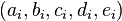 , specifying the matrix
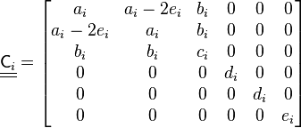
The elastic moduli for the effective medium will be
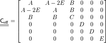
where
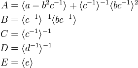
 denotes the volume weighted average over all layers.
This includes isotropic layers, as the layer is isotropic if  ,
,  and
and  .
.
Short and medium wavelength approximation
Solutions to wave propagation problems in linear elastic transversely isotropic media can be constructed by superposing solutions for the quasi-P wave, the quasi S-wave, and a S-wave polarized orthogonal to the quasi S-wave.
However, the equations for the angular variation of velocity are algebraically complex and the plane-wave velocities are functions of the propagation angle are.[6] The direction dependent wave speeds for elastic waves through the material can be found by using the Christoffel equation and are given by[7]
![\begin{align}
V_{qP}(\theta) &= \sqrt{\frac{C_{11} \sin^2(\theta) + C_{33}
\cos^2(\theta)+C_{44}+\sqrt{M(\theta)}}{2\rho}} \\
V_{qS}(\theta) &= \sqrt{\frac{C_{11} \sin^2(\theta) + C_{33}
\cos^2(\theta)+C_{44}-\sqrt{M(\theta)}}{2\rho}} \\
V_{S} &= \sqrt{\frac{C_{66} \sin^2(\theta) +
C_{44}\cos^2(\theta)}{\rho}} \\
M(\theta) &= \left[\left(C_{11}-C_{44}\right) \sin^2(\theta) - \left(C_{33}-C_{44}\right)\cos^2(\theta)\right]^2
+ \left(C_{13} + C_{44}\right)^2 \sin^2(2\theta) \\
\end{align}](../I/m/3240332e7afb09df3af4fefe391ed08c.png)
where  is the angle between the axis of symmetry and the wave propagation direction,
  is mass density and the are elements of the elastic stiffness matrix. The Thomsen parameters are used to simplify these expressions and make them easier to understand.
Thomsen parameters
Thomsen parameters[8] are dimensionless combinations of elastic moduli which characterize transversely isotropic materials, that are encountered, for example, in geophysics. In terms of the components of the elastic stiffness matrix, these parameters are defined as:
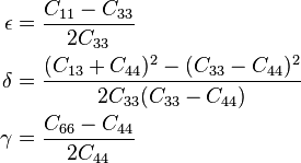
where index 3 indicates the axis of symmetry ( ) . These parameters, in conjunction with the associated P wave and S wave velocities, can be used to characterize wave propagation through weakly anisotropic, layered media. It is found empirically that, for most layered rock formations the Thomsen parameters are usually much less than 1.
The name refers to Leon Thomsen, professor of geophysics at the University of Houston, who proposed these parameters in his 1986 paper "Weak Elastic Anisotropy".
Simplified expressions for wave velocities
In geophysics the anisotropy in elastic properties is usually weak, in which case  . When the exact expressions for the wave velocities above are linearized in these small quantities, they simplify to
![\begin{align}
V_{qP}(\theta) & \approx V_{P0}(1 + \delta \sin^2 \theta \cos^2 \theta + \epsilon \sin^4 \theta) \\
V_{qS}(\theta) & \approx V_{S0}\left[1 + \left(\frac{V_{P0}}{ V_{S0}}\right)^2(\epsilon-\delta) \sin^2 \theta \cos^2 \theta\right] \\
V_{S}(\theta) & \approx V_{S0}(1 + \gamma \sin^2 \theta )
\end{align}](../I/m/bec505a24c7d20ae3adf9aea77ec3b7f.png)
where
are the P and S wave velocities in the direction of the axis of symmetry () (in geophysics, this is usually, but not always, the vertical direction). Note that  may be further linearized, but this does not lead to further simplification.
The approximate expressions for the wave velocities are simple enough to be physically interpreted, and sufficiently accurate for most geophysical applications. These expressions are also useful in some contexts where the anisotropy is not weak.
See also
References
- ↑ Milton, G. W. (2002). The Theory of Composites. Cambridge University Press. doi:10.2277/0521781256.
- ↑ Slawinski, M. A. (2010). Waves and Rays in Elastic Continua. World Scientific.
- ↑ We can use the values and for a derivation of the stiffness matrix for transversely isotropic materials. Specific values are chosen to make the calculation easier.
- ↑ 4.0 4.1 Backus, G. E. (1962), Long-Wave Elastic Anisotropy Produced by Horizontal Layering, J. Geophys. Res., 67(11), 4427–4440
- ↑ Ikelle, Luc T. and Amundsen, Lasse (2005),Introduction to petroleum seismology, SEG Investigations in Geophysics No. 12
- ↑ Nye, J. F. (2000). Physical Properties of Crystals: Their Representation by Tensors and Matrices. Oxford University Press.
- ↑ G. Mavko, T. Mukerji, J. Dvorkin. The Rock Physics Handbook. Cambridge University Press 2003 (paperback). ISBN 0-521-54344-4
- ↑ Thomsen, Leon (1986). "Weak Elastic Anisotropy". Geophysics 51 (10): 1954–1966. Bibcode:1986Geop...51.1954T. doi:10.1190/1.1442051.