Total variation denoising

Example of application of the Rudin et al.^[1] total variation denoising technique to an image corrupted by Gaussian noise. This example created using demo_tv.m by Guy Gilboa, see external links.

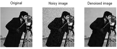
In signal processing, Total variation denoising, also known as total variation regularization is a process, most often used in digital image processing, that has applications in noise removal. It is based on the principle that signals with excessive and possibly spurious detail have high total variation, that is, the integral of the absolute gradient of the signal is high. According to this principle, reducing the total variation of the signal subject to it being a close match to the original signal, removes unwanted detail whilst preserving important details such as edges. The concept was pioneered by Rudin et al. in 1992.^[1]

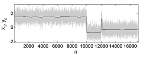
This noise removal technique has advantages over simple techniques such as linear smoothing or median filtering which reduce noise but at the same time smooth away edges to a greater or lesser degree. By contrast, total variation denoising is remarkably effective at simultaneously preserving edges whilst smoothing away noise in flat regions, even at low signal-to-noise ratios.^[2]

Mathematical exposition for 1D digital signals

Application of 1D total variation denoising to a signal obtained from a single-molecule experiment.^[3] Gray is the original signal, black is the denoised signal.

For a digital signal $y_n$ , we can, for example, define the total variation as:

V(y) = \sum\limits_n\left|y_{n+1}-y_n \right|

Given an input signal $x_n$ , the goal of total variation denoising is to find an approximation, call it $y_n$ , that has smaller total variation than $x_n$ but is "close" to $x_n$ . One measure of closeness is the sum of square errors:

E(x,y) = \frac{1}{2}\sum\limits_n\left(x_n - y_n\right)^2

So the total variation denoising problem amounts to minimizing the following discrete functional over the signal $y_n$ :

E(x,y) + \lambda V(y)

By differentiating this functional with respect to $y_n$ , we can derive a corresponding Euler–Lagrange equation, that can be numerically integrated with the original signal $x_n$ as initial condition. This was the original approach.^[1] Alternatively, since this is a convex functional, techniques from convex optimization can be used to minimize it and find the solution $y_n$ .^[3]

Regularization properties

The regularization parameter $\lambda$ plays a critical role in the denoising process. When $\lambda=0$ , there is no denoising and the result is identical to the input signal. As $\lambda \to \infty$ , however, the total variation term plays an increasingly strong role, which forces the result to have smaller total variation, at the expense of being less like the input (noisy) signal. Thus, the choice of regularization parameter is critical to achieving just the right amount of noise removal.

2D digital signals

We now consider 2D signals y, such as images. The total variation norm proposed by the 1992 paper is

V(y) = \sum_{i,j} \sqrt{ |y_{i+1,j} - y_{i,j}|^2 + |y_{i,j+1} - y_{i,j}|^2 }

and is isotropic and not differentiable. A variation that is sometimes used, since it may sometimes be easier to minimize, is an anisotropic version

V_\text{aniso}(y) = \sum_{i,j} \sqrt{ |y_{i+1,j} - y_{i,j}|^2} + \sqrt{|y_{i,j+1} - y_{i,j}|^2 } = \sum_{i,j} |y_{i+1,j} - y_{i,j}| + |y_{i,j+1} - y_{i,j}|.

The standard total variation denoising problem is still of the form

\min_y \; E(x,y) + \lambda V(y)

where E is the 2D L2 norm. In contrast to the 1D case, solving this denoising is non-trivial. A recent algorithm that solves this is known as Chambolle's Algorithm.^[4]

Due in part to much research in compressed sensing in the mid-2000s, there are many algorithms, such as the split-Bregman method, that solve variants of this problem.

External links

References

↑ 1.0 1.1 1.2 Rudin, L. I.; Osher, S.; Fatemi, E. (1992). "Nonlinear total variation based noise removal algorithms". Physica D 60: 259–268. doi:10.1016/0167-2789(92)90242-f.
↑ Strong, D.; Chan, T. (2003). "Edge-preserving and scale-dependent properties of total variation regularization". Inverse Problems 19: S165–S187. doi:10.1088/0266-5611/19/6/059.
↑ 3.0 3.1 Little, M. A.; Jones, Nick S. (2010). "Sparse Bayesian Step-Filtering for High-Throughput Analysis of Molecular Machine Dynamics". ICASSP 2010 Proceedings. 2010 IEEE International Conference on Acoustics, Speech and Signal Processing.
↑ Chambolle, A. (2004). "An algorithm for total variation minimization and applications". Journal of Mathematical Imaging and Vision 20: 89–97. doi:10.1023/B:JMIV.0000011325.36760.1e. CiteSeerX: 10.1.1.160.5226.