Tomasi–Kanade factorization
The Tomasi–Kanade factorization is the seminal work by Carlo Tomasi and Takeo Kanade in the early 1990s.[1] It charted out an elegant and simple solution based on a SVD-based factorization scheme for analysing image measurements of a rigid object captured from different views using a weak perspective camera model. The crucial observation made by authors was that if all the measurements (i.e., image co-ordinates of all the points in all the views) are collected in a single matrix, the point trajectories will reside in a certain subspace. The dimension of the subspace in which the image data resides is a direct consequence of two factors:
- The type of camera that projects the scene (for example, affine or perspective)
- The nature of inspected object (for instance, rigid or non-rigid).
The low-dimensionality of the subspace is mirrored (captured) trivially as reduced rank of the measurement matrix. This reduced rank of measurement matrix can be motivated from the fact that, the position of the projection of an object point on the image plane is constrained as the motion of each point is globally described by a precise geometric model.
Method
The rigid-body factorization introduced in provides a description of 3D structure of a rigid object in terms of a set of feature points extracted from salient image features. After tracking the points throughout all the images composing the temporal sequence, a set of trajectories is available. These trajectories are constrained globally at each frame by the rigid transformation which the shape is undergoing, i.e., trajectory of every point will have similar profile.
Let the location of a point j in a frame i be defined as pij = (xij, yij)T where xij and yij are horizontal and vertical image co-ordinates respectively .
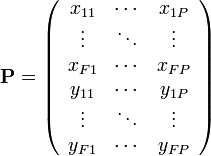
A compact representation of the image measurements can be expressed by collecting all the non-homogeneous co-ordinates in a single matrix, called the observation matrix P such that
P is a 2F × P matrix, where F is the number of frames and P the number of feature points. Ideally, the observation matrix, should contain perfect information about the object being tracked. Unfortunately, in practice, most state-of-art trackers can only provide point tracks that are incomplete (due to occlusion) and inaccurate (due to sensor noise) if placed in an unstructured environment.
As mentioned earlier, the central premise behind the factorization approach is that a measurement matrix P is rank limited. Further, it is possible to factor P into two sub-matrices: a motion and a shape matrix, M and S of size 2F × r and N × r respectively.
The size and structure of S generally depends on the shape properties (for example whether it is rigid or non-rigid) and M depends both on the type of camera model we assume and the shape properties. The essence of factorization method is computing
The optimal r-rank approximation of P with respect to the Frobenius norm can be found out using a SVD-based scheme.
References
- ↑ Carlo Tomasi and Takeo Kanade. (November 1992). "Shape and motion from image streams under orthography: a factorization method.". International Journal of Computer Vision, 9 (2): 137–154. doi:10.1007/BF00129684.

