Tetradic Palatini action

Main article: Frame fields in general relativity

The Einstein–Hilbert action for general relativity was first formulated purely in terms of the space-time metric. To take the metric and affine connection as independent variables in the action principle was first considered by Palatini.^[1] It is called a first order formulation as the variables to vary over involve only up to first derivatives in the action and so doesn't over complicate the Euler–Lagrange equations with terms coming from higher derivative terms. The tetradic Palatini action is another first-order formulation of the Einstein–Hilbert action in terms of a different pair of independent variables, known as frame fields and the spin connection. The use of frame fields and spin connections are essential in the formulation of a generally covariant fermionic action (see the article spin connection for more discussion of this) which couples fermions to gravity when added to the tetradic Palatini action.

Not only is this needed to couple fermions to gravity and makes the tetradic action somehow more fundamental to the metric version, the Palatini action is also a stepping stone to more interesting actions like the self-dual Palatini action which can be seen as the Lagrangian basis for Ashtekar's formulation of canonical gravity (see Ashtekar's variables) or the Holst action which is the basis of the real variables version of Ashtekar's theory. Another important action is the Plebanski action (see the entry on the Barrett–Crane model), and proving that it gives general relativity under certain conditions involves showing it reduces to the Palatini action under these conditions.

Here we present definitions and calculate Einstein's equations from the Palatini action in detail. These calculations can be easily modified for the self-dual Palatini action and the Holst action.

Some definitions

We first need to introduce the notion of tetrads. A tetrad is an orthonormal vector basis in terms of which the space-time metric looks locally flat,

$g_{\alpha \beta} = e_\alpha^I e_\beta^J \eta_{IJ}$

where $\eta_{IJ} = diag (-1,1,1,1)$ is the Minkowski metric. The tetrads encode the information about the space-time metric and will be taken as one of the independent variables in the action principle.

Now if one is going to operate on objects that have internal indices one needs to introduce an appropriate derivative (covariant derivative). We introduce an arbitrary covariant derivative via

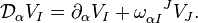
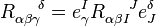
$\mathcal{D}_\alpha V_I = \partial_\alpha V_I + \omega_{\alpha I}^{\;\;\;\; J} V_J .$

Where $\omega_{\alpha I}^{\;\;\;\; J}$ is a Lorentz connection (the derivative annihilates the Minkowski metric $\eta_{IJ}$ ). We define a curvature via

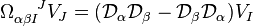
$\Omega_{\alpha \beta I}^{\;\;\;\;\;\; J} V_J = (\mathcal{D}_\alpha \mathcal{D}_\beta - \mathcal{D}_\beta\mathcal{D}_\alpha) V_I$

We obtain

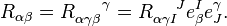
${\Omega_{\alpha \beta}}^{IJ} = 2 \partial_{[\alpha} {\omega_{\beta]}}^{IJ} + 2 {\omega_{[\alpha}}^{IK} {\omega_{\beta] K}}^J$ .

We introduce the covariant derivative which annihilates the tetrad,

$\nabla_\alpha e_\beta^I = 0$ .

The connection is completely determined by the tetrad. The action of this on the generalized tensor $V_\beta^I$ is given by

$\nabla_\alpha V_\beta^I = \partial_\alpha V_\beta^I - \Gamma_{\alpha \beta}^\gamma V_\gamma^I - \Gamma_{\alpha \; J}^{\;\; I} V_\beta^J.$

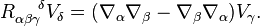
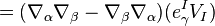
We define a curvature $R_{\alpha \beta}^{\;\;\;\; IJ}$ by

$R_{\alpha \beta I}^{\;\;\;\;\;\; J} V_J = (\nabla_\alpha \nabla_\beta - \nabla_\beta \nabla_\alpha) V_I$ .

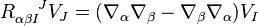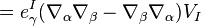
This is easily related to the usual curvature defined by

$R_{\alpha \beta \gamma}^{\;\;\;\;\;\; \delta} V_\delta = (\nabla_\alpha \nabla_\beta - \nabla_\beta \nabla_\alpha) V_\gamma$

via substituting $V_\gamma = V_I e^I_\gamma$ into this expression (see below for details). One obtains,

$R_{\alpha \beta \gamma}^{\;\;\;\;\;\; \delta} = e_\gamma^I R_{\alpha \beta I}^{\;\;\;\;\;\; J} e_J^\delta , \quad R_{\alpha \beta} = R_{\alpha \gamma I}^{\;\;\;\;\;\; J} e^I_\beta e^\gamma_J \;\; and \;\; R = R_{\alpha \beta}^{\;\;\;\; IJ} e_I^\alpha e_J^\beta$

for the Riemann tensor, Ricci tensor and Ricci scalar respectively.

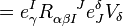
The tetradic Palatini action

The Ricci scalar of this curvature can be expressed as $e^\alpha_I e^\beta_J \Omega_{\alpha \beta}^{\;\;\;\; IJ}$ . The action can be written

$S_{H-P} = \int d^4 x \; e \; e^\alpha_I e^\beta_J \Omega_{\alpha \beta}^{\;\;\;\; IJ}$

where $e = \sqrt{-g}$ but now $g$ is a function of the frame field.

We will derive the Einstein equations by varying this action with respect to the tetrad and spin connection as independent quantities.

As a shortcut to performing the calculation we introduce a connection compatible with the tetrad, $\nabla_\alpha e^I_\beta = 0.$ ^[2] The connection associated with this covariant derivative is completely determined by the tetrad. The difference between the two connections we have introduced is a field $C_{\alpha I}^{\;\;\; J}$ defined by

$C_{\alpha I}^{\;\;\; J} V_J = (D_\alpha - \nabla_\alpha) V_I.$

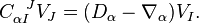
We can compute the difference between the curvatures of these two covariant derivatives (see below for details),

$\Omega_{\alpha \beta}^{\;\;\;\; IJ} - R_{\alpha \beta}^{\;\;\;\; IJ} = \nabla_{[\alpha} C_{\beta]}^{\;\; IJ} + C_{[\alpha}^{\;\;\; IM} C_{\beta]M}^{\;\;\;\; J}$

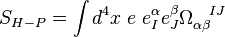
The reason for this intermediate calculation is that it is easier to compute the variation by reexpressing the action in terms of $\nabla$ and $C_\alpha^{\;\; IJ}$ and noting that the variation with respect to $\omega_\alpha^{\;\;\; IJ}$ is the same as the variation with respect to $C_\alpha^{\;\; IJ}$ (when keeping the tetrad fixed). The action becomes

$S_{H-P} = \int d^4x \; e \; e^\alpha_I e^\beta_J (R_{\alpha \beta}^{\;\;\;\; IJ} + \nabla_{[\alpha} C_{\beta]}^{\;\; IJ} + C_{[\alpha}^{\;\;\; IM} C_{\beta]M}^{\;\;\;\; J})$

We first vary with respect to $C_\alpha^{\;\; IJ}$ . The first term does not depend on $C_\alpha^{\;\; IJ}$ so it does not contribute. The second term is a total derivative. The last term yields $e^{[a}_M e^{b]}_N \delta^M_{[I} \delta^K_{J]} C_{bK}^{\;\;\; N} = 0$ . We show below that this implies that $C_\alpha^{\;\; IJ} = 0$ as the prefactor $e^{[a}_M e^{b]}_N \delta^M_{[I} \delta^K_{J]}$ is non-degenerate. This tells us that $\nabla$ coincides with $D$ when acting on objects with only internal indices. Thus the connection $D$ is completely determined by the tetrad and $\Omega$ coincides with $R$ . To compute the variation with respect to the tetrad we need the variation of $e = \det e_\alpha^I$ . From the standard formula

$\delta \det (a) = \det (a) (a^{-1})_{ji} \delta a_{ij}$

we have $\delta e = e e_I^\alpha \delta e_\alpha^I$ . Or upon using $\delta (e_\alpha^I e_I^\alpha) = 0$ , this becomes $\delta e = - e e_\alpha^I \delta e_I^\alpha$ . We compute the second equation by varying with respect to the tetrad,

$\delta S_{H-P} = \int d^4 x \; e \; \Big( (\delta e^\alpha_I) e^\beta_J \Omega_{\alpha \beta}^{\;\;\;\; IJ} + e^\alpha_I (\delta e^\beta_J) \Omega_{\alpha \beta}^{\;\;\;\; IJ} - e_\gamma^K (\delta e_K^\gamma) e^\alpha_I e^\beta_J \Omega_{\alpha \beta}^{\;\;\;\; IJ} \Big)$

$\;\;\;\;\; = 2 \int d^4 x \; e \; \Big( e^\beta_J \Omega_{\alpha \beta}^{\;\;\;\; IJ} - {1 \over 2} e_M^\gamma e_N^\delta e_\alpha^I \Omega_{\gamma \delta}^{\;\;\;\; MN} \Big) (\delta e_I^\alpha)$

One gets, after substituting $\Omega_{\alpha \beta}^{\;\;\;\; IJ}$ for $R_{\alpha \beta}^{\;\;\;\; IJ}$ as given by the previous equation of motion,

$e_J^\gamma R_{\alpha \gamma}^{\;\;\;\; IJ} - {1 \over 2} R_{\gamma \delta}^{\;\;\;\; MN} e_M^\gamma e_N^\delta e_\alpha^I = 0$

which, after multiplication by $e_{I \beta}$ just tells us that the Einstein tensor 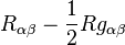$R_{\alpha \beta} - {1 \over 2} R g_{\alpha \beta}$ of the metric defined by the tetrads vanishes. We have therefore proved that the Palatini variation of the action in tetradic form yields the usual Einstein equations.

Generalizations of the Palatini action

Main articles: Holst action, Self-dual Palatini action, Barbero-Immirzi parameter and Plebanski action

We change the action by adding a term

$- {1 \over 2 \gamma} e e_I^\alpha e_J^\beta \Omega_{\alpha \beta}^{\;\;\;\; MN} [\omega] \epsilon^{IJ}_{\;\;\; MN}$

This modifies the Palatini action to

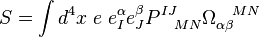
$S = \int d^4 x \; e \; e^\alpha_I e^\beta_J P^{IJ}_{\;\;\;\; MN} \Omega_{\alpha \beta}^{\;\;\;\; MN}$

where

$P^{IJ}_{\;\;\;\; MN} = \delta_M^{[I} \delta_N^{J]} - {1 \over 2 \gamma} \epsilon^{IJ}_{\;\;\; MN}.$

This action given above is the Holst action, introduced by Holst^[3] and $\gamma$ is the Barbero-Immirzi parameter whose role was recognized by Barbero^[4] and Immirizi.^[5] The self dual formulation corresponds to the choice $\gamma = -i$ .

It is easy to show these actions give the same equations. However, the case corresponding to $\gamma = \pm i$ must be done separately (see article self-dual Palatini action). Assume $\gamma \not= \pm i$ , then $P^{IJ}_{\;\;\;\; MN}$ has an inverse given by

$(P^{-1})_{IJ}^{\;\;\;\; MN} = {\gamma^2 \over \gamma^2 + 1} \Big( \delta_I^{[M} \delta_J^{N]} + {1 \over 2 \gamma} \epsilon_{IJ}^{\;\;\; MN} \Big).$

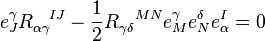
(note this diverges for $\gamma = \pm i$ ). As this inverse exists the generalization of the prefactor $e^{[a}_M e^{b]}_N \delta^M_{[I} \delta^K_{J]}$ will also be non-degenerate and as such equivalent conditions are obtained from variation with respect to the connection. We again obtain $C_\alpha^{\;\; IJ} = 0$ . While variation with respect to the tetrad yields Einstein's equation plus an additional term. However, this extra term vanishes by symmetries of the Riemann tensor.

Details of calculation

Relating usual curvature to the mixed index curvature

The usual Riemann curvature tensor $R_{\alpha \beta \gamma}^{\;\;\;\;\;\; \delta}$ is defined by

$R_{\alpha \beta \gamma}^{\;\;\;\;\;\; \delta} V_\delta = (\nabla_\alpha \nabla_\beta - \nabla_\beta \nabla_\alpha) V_\gamma.$

To find the relation to the mixed index curvature tensor let us substitute $V_\gamma = e_\gamma^I V_I$

$R_{\alpha \beta \gamma}^{\;\;\;\;\;\; \delta} V_\delta = (\nabla_\alpha \nabla_\beta - \nabla_\beta \nabla_\alpha) V_\gamma$

$= (\nabla_\alpha \nabla_\beta - \nabla_\beta \nabla_\alpha) (e_\gamma^I V_I)$

$= e_\gamma^I (\nabla_\alpha \nabla_\beta - \nabla_\beta \nabla_\alpha) V_I$

$= e_\gamma^I R_{\alpha \beta I}^{\;\;\;\;\;\; J} e_J^\delta V_\delta$

where we have used $\nabla_\alpha e_\beta^I = 0$ . Since this is true for all $V_\delta$ we obtain

$R_{\alpha \beta \gamma}^{\;\;\;\;\;\; \delta} = e_\gamma^I R_{\alpha \beta I}^{\;\;\;\;\;\; J} e_J^\delta$ .

Using this expression we find

$R_{\alpha \beta} = R_{\alpha \gamma \beta}^{\;\;\;\;\;\;\; \gamma} = R_{\alpha \gamma I}^{\;\;\;\;\;\; J} e_\beta^I e_J^\gamma.$

Contracting over $\alpha$ and $\beta$ allows us write the Ricci scalar

$R = R_{\alpha \beta}^{\;\;\;\; IJ} e_I^\alpha e_J^\beta.$

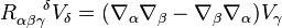
Difference between curvatures

The derivative defined by $D_\alpha V_I$ only knows how to act on internal indices. However, we find it convenient to consider a torsion-free extension to spacetime indices. All calculations will be independent of this choice of extension. Applying $\mathcal{D}_a$ twice on $V_I$ ,

$\mathcal{D}_\alpha \mathcal{D}_\beta V_I = \mathcal{D}_\alpha (\nabla_\beta V_I + C_{\beta I}^{\;\;\; J} V_J)$

$= \nabla_\alpha (\nabla_\beta V_I + C_{\beta I}^{\;\;\; J} V_J) + C_{\alpha I}^{\;\;\; K} (\nabla_b V_K + C_{\beta K}^{\;\;\; J} V_J) + \overline{\Gamma}_{\alpha \beta}^\gamma (\nabla_\gamma V_I + C_{\gamma I}^{\;\;\; J} V_J)$

where $\overline{\Gamma}_{\alpha \beta}^\gamma$ is unimportant, we need only note that it is symmetric in $\alpha$ and $\beta$ as it is torsion-free. Then

$\Omega_{\alpha \beta I}^{\;\;\;\;\;\; J} V_J = (\mathcal{D}_\alpha \mathcal{D}_\beta - \mathcal{D}_\beta \mathcal{D}_\alpha) V_I$

$= (\nabla_\alpha \nabla_\beta - \nabla_\beta \nabla_\alpha) V_I + \nabla_\alpha (C_{\beta I}^{\;\;\; J} V_J) - \nabla_\beta (C_{\alpha I}^{\;\;\; J} V_J)$

$+ \; C_{\alpha I}^{\;\;\; K} \nabla_\beta V_K - C_{\beta I}^{\;\;\; K} \nabla_\alpha V_K + C_{\alpha I}^{\;\;\; K} C_{\beta K}^{\;\;\; J} V_J - C_{\beta I}^{\;\;\; K} C_{\alpha K}^{\;\;\; J} V_J$

$= R_{\alpha \beta I}^{\;\;\;\;\; J} V_J + (\nabla_\alpha C_{\beta I}^{\;\;\; J} - \nabla_\beta C_{\alpha I}^{\;\;\; J} + C_{\alpha I}^{\;\;\; K} C_{\beta K}^{\;\;\; J} - C_{\beta_I}^{\;\;\; K} C_{\alpha K}^{\;\;\; J}) V_J$

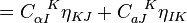
Hence

$\Omega_{ab}^{\;\;\;\; IJ} - R_{ab}^{\;\;\;\; IJ} = 2 \nabla_{[a} C_{b]}^{\;\;\; IJ} + 2 C_{[a}^{\;\;\; IK} C_{b] K}^{\;\;\;\;\; J}$

Varying the action with respect to the field $C_\alpha^{\;\; IJ}$

We would expect $\nabla_a$ to also annihilate the Minkowski metric $\eta_{IJ} = e_{\beta I} e^\beta_J$ . If we also assume that the covariant derivative $\mathcal{D}_\alpha$ annihilates the Minkowski metric (then said to be torsion-free) we have,

$0 = (\mathcal{D}_\alpha - \nabla_\alpha) \eta_{IJ}$

$= C_{\alpha I}^{\;\;\; K} \eta_{KJ} + C_{aJ}^{\;\;\; K} \eta_{IK}$

$= C_{\alpha IJ} + C_{\alpha JI} .$

Implying $C_{\alpha IJ} = C_{\alpha [IJ]}$ .

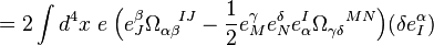
From the last term of the action we have from varying with respect to $C_{\alpha I}^{\;\;\;\; J}$ ,

$\delta S_{EH} = \delta \int d^4 x \; e \; e_M^\gamma e_N^\beta C_{[\gamma}^{\;\;\; MK} C_{\beta]K}^{\;\;\;\; N}$

$= \delta \int d^4 x \; e \; e_M^{[\gamma} e_N^{\beta]} C_\gamma^{\;\;\; MK} C_{\beta K}^{\;\;\;\; N}$

$= \delta \int d^4 x \; e \; e^{M [\gamma} e^{\beta]}_N C_{\gamma M}^{\;\;\;\; K} C_{\beta K}^{\;\;\;\;\; N}$

$= \int d^4 x \; e e^{M [\gamma} e^{\beta]}_N \big( \delta_\gamma^\alpha \delta^I_M \delta^K_J C_{\beta K}^{\;\;\;\;\; N} + C_{\gamma M}^{\;\;\;\; K} \delta^\alpha_\beta \delta^I_K \delta^N_J \big) \delta C_{\alpha I}^{\;\;\;\; J}$

$= \int d^4 x \; e (e^{I [\alpha} e^{\beta]}_N C_{\beta J}^{\;\;\;\; N} + e^{M [\beta} e^{\alpha]}_J C_{\beta M}^{\;\;\;\; I}) \delta C_{\alpha I}^{\;\;\;\; J}$

$e_I^{[\alpha} e^{\beta]}_K C_{\beta J}^{\;\;\;\; K} + e^{K [\beta} e^{\alpha]}_J C_{\beta KI} = 0$

$C_{\beta I}^{\;\;\; K} e^{[\alpha}_K e^{\beta]}_J + C_{\beta J}^{\;\;\; K} e^{[\alpha}_I e^{\beta]}_K = 0 .$

where we have used $C_{\beta KI} = - C_{\beta IK}$ . This can be written more compactly as

$e^{[\alpha}_M e^{\beta]}_N \delta^M_{[I} \delta^K_{J]} C_{\beta K}^{\;\;\; N} = 0 .$

Vanishing of $C_\alpha^{\;\; IJ}$

We will show following the reference "Geometrodynamics vs. Connection Dynamics"^[6] that

$C_{\beta I}^{\;\;\; K} e^{[\alpha}_K e^{\beta]}_J + C_{\beta J}^{\;\;\; K} e^{[\alpha}_I e^{\beta]}_K = 0 \;\;\; Eq. 1$

implies $C_{\alpha I}^{\;\;\;\; J} = 0$ . First we define the spacetime tensor field by

$S_{\alpha \beta \gamma} := C_{\alpha IJ} e^I_\beta e^J_\gamma .$

Then the condition $C_{\alpha IJ} = C_{\alpha [IJ]}$ is equivalent to $S_{\alpha \beta \gamma} = S_{\alpha [\beta \gamma]}$ . Contracting Eq. 1 with $e_\alpha^I e_\gamma^J$ one calculates that

$C_{\beta J}^{\;\;\;\; I} e_\gamma^J e_I^\beta = 0.$

As $S_{\alpha \beta}^{\;\;\;\; \gamma} = C_{\alpha I}^{\;\;\; J} e_\beta^I e_J^\gamma$ , we have $S_{\beta \gamma}^{\;\;\;\; \beta} = 0$ . We write it as

$(C_{\beta I}^{\;\;\; J} e_J^\beta) e_\gamma^I = 0,$

and as $e_\alpha^I$ are invertible this implies

$C_{\beta I}^{\;\;\; J} e_J^\beta = 0.$

Thus the terms $C_{\beta I}^{\;\;\; K} e^\beta_K e^\alpha_J,$ and $C_{\beta J}^{\;\;\; K} e^\alpha_I e^\beta_K$ of Eq. 1 both vanish and Eq. 1 reduces to

$C_{\beta I}^{\;\;\; K} e^\alpha_K e^\beta_J - C_{\beta J}^{\;\;\; K} e^\beta_I e^\alpha_K = 0 .$

If we now contract this with $e^I_\gamma e^J_\delta$ , we get

$0 = (C_{\beta I}^{\;\;\; K} e^\alpha_K e^\beta_J - C_{\beta J}^{\;\;\; K} e^\beta_I e^\alpha_K) e^I_\gamma e^J_\delta$

$= C_{\beta I}^{\;\;\; K} e^\alpha_K e^I_\gamma \delta_\delta^\beta - C_{\beta J}^{\;\;\; K} \delta_\gamma^\beta e^\alpha_K e^J_\delta$

$= C_{\delta I}^{\;\;\; K} e^I_\gamma e^\alpha_K - C_{\gamma J}^{\;\;\; K} e^J_\delta e^\alpha_K$

$S_{\gamma \delta}^{\;\;\; \alpha} = S_{(\gamma \delta)}^{\;\;\;\;\;\; \alpha} .$

Since we have $S_{\alpha \beta \gamma} = S_{\alpha [\beta \gamma]}$ and $S_{\alpha \beta \gamma} = S_{(\alpha \beta) \gamma}$ , we can successively interchange the first two and then last two indices with appropriate sign change each time to obtain,

$S_{\alpha \beta \gamma} = S_{\beta \alpha \gamma} = - S_{\beta \gamma \alpha} = - S_{\gamma \beta \alpha} = S_{\gamma \alpha \beta} = S_{\alpha \gamma \beta} = - S_{\alpha \beta \gamma}$

Implying $S_{\alpha \beta \gamma} = 0$ , or

$C_{\alpha IJ} e_\beta^I e_\gamma^J = 0 ,$

and since the $e_\alpha^I$ are invertible, we get $C_{\alpha IJ} = 0$ . This is the desired result.

References

↑ A. Palatini (1919) Deduzione invariantiva delle equazioni gravitazionali dal principio di Hamilton, Rend. Circ. Mat. Palermo 43, 203-212 [English translation by R.Hojman and C. Mukku in P.G. Bergmann and V. De Sabbata (eds.) Cosmology and Gravitation, Plenum Press, New York (1980)]
↑ A. Ashtekar "Lectures on non-perturbative canonical gravity" (with invited contributions), Bibliopolis, Naples 19988.
↑ Holst, S. (1996). Barbero's Hamilitonian derived from a generalized Hilbert-Palatini action. Phys. Rev. D, 53, 5966-5969.
↑ Barbero G., J.F. (1995), Real Ashtekar variables for Lorentzian signature space-times. Phys. Rev. D, 51(10), 5507-5510.
↑ Immirizi, G. (1997). Real and complex connections for canonical gravity. Class. Quantum Grav., 14, L177-L181.
↑ Geometrodynamics vs. Connection Dynamics, Joseph D. Romano, Gen.Rel.Grav. 25 (1993) 759-854