Tent map

Graph of tent map function

In mathematics, the tent map with parameter μ is the real-valued function f_μ defined by

f_\mu:=\mu\min\{x,\,1-x\},

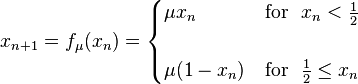
the name being due to the tent-like shape of the graph of f_μ. For the values of the parameter μ within 0 and 2, f_μ maps the unit interval [0, 1] into itself, thus defining a discrete-time dynamical system on it (equivalently, a recurrence relation). In particular, iterating a point x₀ in [0, 1] gives rise to a sequence $x_n$ :

x_{n+1}=f_\mu(x_n)=\begin{cases} \mu x_n & \mathrm{for}~~ x_n < \frac{1}{2} \\ \\ \mu (1-x_n) & \mathrm{for}~~ \frac{1}{2} \le x_n \end{cases}

where μ is a positive real constant. Choosing for instance the parameter μ=2, the effect of the function f_μ may be viewed as the result of the operation of folding the unit interval in two, then stretching the resulting interval [0,1/2] to get again the interval [0,1]. Iterating the procedure, any point x₀ of the interval assumes new subsequent positions as described above, generating a sequence x_n in [0,1].

The $\mu=2$ case of the tent map is a non-linear transformation of both the bit shift map and the r=4 case of the logistic map.

Behaviour

Orbits of unit-height tent map

Bifurcation diagram for the tent map. Higher density indicates increased probability of the x variable acquiring that value for the given value of the μ parameter.

The tent map and the logistic map are topologically conjugate,^[1] and thus the behaviours of the two maps are in this sense identical under iteration.

Depending on the value of μ, the tent map demonstrates a range of dynamical behaviour ranging from predictable to chaotic.

If μ is less than 1 the point x = 0 is an attractive fixed point of the system for all initial values of x i.e. the system will converge towards x = 0 from any initial value of x.
If μ is 1 all values of x less than or equal to 1/2 are fixed points of the system.
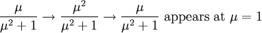
If μ is greater than 1 the system has two fixed points, one at 0, and the other at μ/(μ + 1). Both fixed points are unstable i.e. a value of x close to either fixed point will move away from it, rather than towards it. For example, when μ is 1.5 there is a fixed point at x = 0.6 (because 1.5(1 − 0.6) = 0.6) but starting at x = 0.61 we get

0.61 \to 0.585 \to 0.6225 \to 0.56625 \to 0.650625 \ldots

If μ is between 1 and the square root of 2 the system maps a set of intervals between μ − μ²/2 and μ/2 to themselves. This set of intervals is the Julia set of the map i.e. it is the smallest invariant sub-set of the real line under this map. If μ is greater than the square root of 2, these intervals merge, and the Julia set is the whole interval from μ − μ²/2 to μ/2 (see bifurcation diagram).
If μ is between 1 and 2 the interval [μ − μ²/2, μ/2]contains both periodic and non-periodic points, although all of the orbits are unstable (i.e. nearby points move away from the orbits rather than towards them). Orbits with longer lengths appear as μ increases. For example:

\frac{\mu}{\mu^2+1} \to \frac{\mu^2}{\mu^2+1} \to \frac{\mu}{\mu^2+1} \mbox{ appears at } \mu=1

\frac{\mu}{\mu^3+1} \to \frac{\mu^2}{\mu^3+1} \to \frac{\mu^3}{\mu^3+1} \to \frac{\mu}{\mu^3+1} \mbox{ appears at } \mu=\frac{1+\sqrt{5}}{2}

\frac{\mu}{\mu^4+1} \to \frac{\mu^2}{\mu^4+1} \to \frac{\mu^3}{\mu^4+1} \to \frac{\mu^4}{\mu^4+1} \to \frac{\mu}{\mu^4+1} \mbox{ appears at } \mu \approx 1.8393

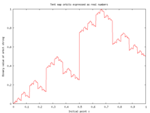
If μ equals 2 the system maps the interval [0,1] onto itself. There are now periodic points with every orbit length within this interval, as well as non-periodic points. The periodic points are dense in [0,1], so the map has become chaotic. In fact, the dynamics will be non-periodic if and only if $x_0$ is irrational. This can be seen by noting what the map does when $x_n$ is expressed in binary notation: It shifts the binary point one place to the right; then, if what appears to the left of the binary point is a "one" it changes all ones to zeroes and vice versa (with the exception of the final bit "one" in the case of a finite binary expansion); starting from an irrational number, this process goes on forever without repeating itself. The invariant measure for x is the uniform density over the unit interval.^[2] The autocorrelation function for a sufficiently long sequence { $x_n$ } will show zero autocorrelation at all non-zero lags.^[3] Thus ${x_n}$ cannot be distinguished from white noise using the autocorrelation function. Note that the r=4 case of the logistic map and the $\mu =2$ case of the tent map are transformations of each other: Denoting the logistically evolving variable as $y_n$ , we have

x_n = \tfrac{2}{\pi}\sin^{-1}(y_{n}^{1/2}).

If μ is greater than 2 the map's Julia set becomes disconnected, and breaks up into a Cantor set within the interval [0,1]. The Julia set still contains an infinite number of both non-periodic and periodic points (including orbits for any orbit length) but almost every point within [0,1] will now eventually diverge towards infinity. The canonical Cantor set (obtained by successively deleting middle thirds from subsets of the unit line) is the Julia set of the tent map for μ = 3.

Magnifying the orbit diagram

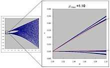
Magnification near the tip shows more details.

A closer look at the orbit diagram shows that there are 4 separated regions at μ ≈ 1. For further magnification, 2 reference lines (red) are drawn from the tip to suitable x at certain μ (e.g., 1.10) as shown.

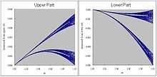
Further magnification shows 8 separated regions.

With distance measured from the corresponding reference lines, further detail appears in the upper and lower part of the map. (total 8 separated regions at some μ)

Asymmetric tent map

The asymmetric tent map is essentially a distorted, but still piecewise linear, version of the $\mu=2$ case of the tent map. It is defined by

$v_{n+1}=\begin{cases} v_n/a &\mathrm{for}~~ v_n \in [0,a) \\ \\ (1-v_n)/(1-a) &\mathrm{for}~~ v_n \in [a,1] \end{cases}$

for parameter $a \in [0,1]$ . The $\mu=2$ case of the tent map is the present case of $a= \tfrac{1}{2}$ . A sequence { $v_n$ } will have the same autocorrelation function ^[3] as will data from the first-order autoregressive process $w_{n+1} = (2a-1)w_n + u_{n+1}$ with { $u_n$ } independently and identically distributed. Thus data from an asymmetric tent map cannot be distinguished, using the autocorrelation function, from data generated by a first-order autoregressive process.

References

↑ Conjugating the Tent and Logistic Maps, Jeffrey Rauch, University of Michigan
↑ Collett, Pierre, and Eckmann, Jean-Pierre, Iterated Maps on the Interval as Dynamical Systems, Boston: Birkhauser, 1980.
↑ 3.0 3.1 Brock, W. A., "Distinguishing random and deterministic systems: Abridged version," Journal of Economic Theory 40, October 1986, 168-195.

External links

ChaosBook.org

Chaos theory

Chaos theory	Anosov diffeomorphism Bifurcation theory Butterfly effect Chaos theory in organizational development Complexity Control of chaos Dynamical system Edge of chaos Fractal Predictability Quantum chaos Santa Fe Institute Synchronization of chaos Unintended consequences

Chaotic maps (list)	Arnold tongue Arnold's cat map Baker's map Complex quadratic map Complex squaring map Coupled map lattice Double pendulum Double scroll attractor Duffing equation Duffing map Dyadic transformation Dynamical billiards outer Exponential map Gauss map Gingerbreadman map Hénon map Horseshoe map Ikeda map Interval exchange map Kaplan–Yorke map Logistic map Lorenz system Multiscroll attractor Rabinovich–Fabrikant equations Rössler attractor Standard map Swinging Atwood's machine Tent map Tinkerbell map Van der Pol oscillator Zaslavskii map

Chaos systems	Bouncing ball dynamics Chua's circuit Economic bubble Tilt-A-Whirl

Chaos theorists	Michael Berry Leon O. Chua Mitchell Feigenbaum Martin Gutzwiller Brosl Hasslacher Michel Hénon Edward Norton Lorenz Aleksandr Lyapunov Benoît Mandelbrot Henri Poincaré Otto Rössler David Ruelle Oleksandr Mykolaiovych Sharkovsky Floris Takens James A. Yorke