Telescoping series

In mathematics, a telescoping series is a series whose partial sums eventually only have a fixed number of terms after cancellation.^[1]^[2] Such a technique is also known as the method of differences.

For example, the series

\sum_{n=1}^\infty\frac{1}{n(n+1)}

simplifies as

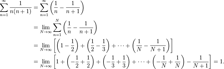
\begin{align} \sum_{n=1}^\infty \frac{1}{n(n+1)} & {} = \sum_{n=1}^\infty \left( \frac{1}{n} - \frac{1}{n+1} \right) \\ {} & {} = \lim_{N\to\infty} \sum_{n=1}^N \left( \frac{1}{n} - \frac{1}{n+1} \right) \\ {} & {} = \lim_{N\to\infty} \left\lbrack {\left(1 - \frac{1}{2}\right) + \left(\frac{1}{2} - \frac{1}{3}\right) + \cdots + \left(\frac{1}{N} - \frac{1}{N+1}\right) } \right\rbrack \\ {} & {} = \lim_{N\to\infty} \left\lbrack { 1 + \left( - \frac{1}{2} + \frac{1}{2}\right) + \left( - \frac{1}{3} + \frac{1}{3}\right) + \cdots + \left( - \frac{1}{N} + \frac{1}{N}\right) - \frac{1}{N+1} } \right\rbrack = 1. \end{align}

In general

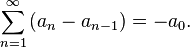
Let $a_n$ be a sequence of numbers. Then,

\sum_{n=1}^N \left(a_n - a_{n-1}\right) = a_N - a_{0},

and, if $a_n \rightarrow 0$

\sum_{n=1}^\infty \left(a_n - a_{n-1}\right) = - a_{0}.

A pitfall

Although telescoping can be a useful technique, there are pitfalls to watch out for:

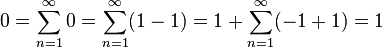
0 = \sum_{n=1}^\infty 0 = \sum_{n=1}^\infty (1-1) = 1 + \sum_{n=1}^\infty (-1 + 1) = 1\,

is not correct because this regrouping of terms is invalid unless the individual terms converge to 0; see Grandi's series. The way to avoid this error is to find the sum of the first N terms first and then take the limit as N approaches infinity:

\begin{align} \sum_{n=1}^N \frac{1}{n(n+1)} & {} = \sum_{n=1}^N \left( \frac{1}{n} - \frac{1}{n+1} \right) \\ & {} = \left(1 - \frac{1}{2}\right) + \left(\frac{1}{2} - \frac{1}{3}\right) + \cdots + \left(\frac{1}{N} -\frac{1}{N+1}\right) \\ & {} = 1 + \left(- \frac{1}{2} + \frac{1}{2}\right) + \left( - \frac{1}{3} + \frac{1}{3}\right) + \cdots + \left(-\frac{1}{N} + \frac{1}{N}\right) - \frac{1}{N+1} \\ & {} = 1 - \frac{1}{N+1}\to 1\ \mathrm{as}\ N\to\infty. \end{align}

More examples

Many trigonometric functions also admit representation as a difference, which allows telescopic cancelling between the consecutive terms.

\begin{align} \sum_{n=1}^N \sin\left(n\right) & {} = \sum_{n=1}^N \frac{1}{2} \csc\left(\frac{1}{2}\right) \left(2\sin\left(\frac{1}{2}\right)\sin\left(n\right)\right) \\ & {} =\frac{1}{2} \csc\left(\frac{1}{2}\right) \sum_{n=1}^N \left(\cos\left(\frac{2n-1}{2}\right) -\cos\left(\frac{2n+1}{2}\right)\right) \\ & {} =\frac{1}{2} \csc\left(\frac{1}{2}\right) \left(\cos\left(\frac{1}{2}\right) -\cos\left(\frac{2N+1}{2}\right)\right). \end{align}

Some sums of the form

\sum_{n=1}^N {f(n) \over g(n)},

where f and g are polynomial functions whose quotient may be broken up into partial fractions, will fail to admit summation by this method. In particular, we have

\begin{align} \sum^\infty_{n=0}\frac{2n+3}{(n+1)(n+2)} & {} =\sum^\infty_{n=0}\left(\frac{1}{n+1}+\frac{1}{n+2}\right) \\ & {} = \left(\frac{1}{1} + \frac{1}{2}\right) + \left(\frac{1}{2} + \frac{1}{3}\right) + \left(\frac{1}{3} + \frac{1}{4}\right) + \cdots \\ & {} \cdots + \left(\frac{1}{n-1} + \frac{1}{n}\right) + \left(\frac{1}{n} + \frac{1}{n+1}\right) + \left(\frac{1}{n+1} + \frac{1}{n+2}\right) + \cdots \\ & {} =\infty. \end{align}

The problem is that the terms do not cancel.

Let k be a positive integer. Then

\sum^\infty_{n=1} {\frac{1}{n(n+k)}} = \frac{H_k}{k}

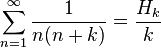
where H_k is the kth harmonic number. All of the terms after 1/(k − 1) cancel.

An application in probability theory

In probability theory, a Poisson process is a stochastic process of which the simplest case involves "occurrences" at random times, the waiting time until the next occurrence having a memoryless exponential distribution, and the number of "occurrences" in any time interval having a Poisson distribution whose expected value is proportional to the length of the time interval. Let X_t be the number of "occurrences" before time t, and let T_x be the waiting time until the xth "occurrence". We seek the probability density function of the random variable T_x. We use the probability mass function for the Poisson distribution, which tells us that

\Pr(X_t = x) = \frac{(\lambda t)^x e^{-\lambda t}}{x!},

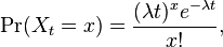
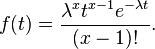
where λ is the average number of occurrences in any time interval of length 1. Observe that the event {X_t ≥ x} is the same as the event {T_x ≤ t}, and thus they have the same probability. The density function we seek is therefore

\begin{align} f(t) & {} = \frac{d}{dt}\Pr(T_x \le t) = \frac{d}{dt}\Pr(X_t \ge x) = \frac{d}{dt}(1 - \Pr(X_t \le x-1)) \\ \\ & {} = \frac{d}{dt}\left( 1 - \sum_{u=0}^{x-1} \Pr(X_t = u)\right) = \frac{d}{dt}\left( 1 - \sum_{u=0}^{x-1} \frac{(\lambda t)^u e^{-\lambda t}}{u!} \right) \\ \\ & {} = \lambda e^{-\lambda t} - e^{-\lambda t} \sum_{u=1}^{x-1} \left( \frac{\lambda^ut^{u-1}}{(u-1)!} - \frac{\lambda^{u+1} t^u}{u!} \right) \end{align}

The sum telescopes, leaving

f(t) = \frac{\lambda^x t^{x-1} e^{-\lambda t}}{(x-1)!}.

Other applications

For other applications, see:

Grandi's series;
Proof that the sum of the reciprocals of the primes diverges, where one of the proofs uses a telescoping sum;
Order statistic, where a telescoping sum occurs in the derivation of a probability density function;
Lefschetz fixed-point theorem, where a telescoping sum arises in algebraic topology;
Homology theory, again in algebraic topology;
Eilenberg–Mazur swindle, where a telescoping sum of knots occurs.
Fundamental theorem of calculus, a continuous analog of telescoping series.

Notes and references

↑ Tom M. Apostol, Calculus, Volume 1, Blaisdell Publishing Company, 1962, pages 422–3
↑ Brian S. Thomson and Andrew M. Bruckner, Elementary Real Analysis, Second Edition, CreateSpace, 2008, page 85