Structure tensor
| Feature detection |
|---|
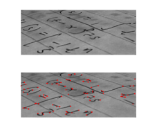 Output of a typical corner detection algorithm |
| Edge detection |
| Corner detection |
| Blob detection |
| Ridge detection |
| Hough transform |
| Structure tensor |
| Affine invariant feature detection |
| Feature description |
| Scale space |
In mathematics, the structure tensor, also referred to as the second-moment matrix, is a matrix derived from the gradient of a function. It summarizes the predominant directions of the gradient in a specified neighborhood of a point, and the degree to which those directions are coherent. The structure tensor is often used in image processing and computer vision.[1][2][3]
The 2D structure tensor
Continuous version
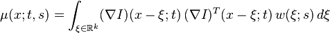
For a function  of two variables p=(x,y), the structure tensor is the 2×2 matrix
![S_w(p) =
\begin{bmatrix}
\int w(r) (I_x(p-r))^2\,d r & \int w(r) I_x(p-r)I_y(p-r)\,d r \\[10pt]
\int w(r) I_x(p-r)I_y(p-r)\,d r & \int w(r) (I_y(p-r))^2\,d r
\end{bmatrix}](../I/m/722a86786a09d85e3a075e3359acd500.png)
where  and
and  are the partial derivatives of with respect to x and y; the integrals range over the plane
  ; and w is some fixed "window function", a distribution on two variables. Note that the matrix
  is itself a function of p=(x,y).
The formula above can be written also as 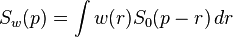 , where
  is the matrix-valued function defined by
![S_0(p)=
\begin{bmatrix}
(I_x(p))^2 & I_x(p)I_y(p) \\[10pt]
I_x(p)I_y(p) & (I_y(p))^2
\end{bmatrix}](../I/m/b5b2846256868862de98bd27d2ae9788.png)
If the gradient 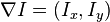 of is viewed as a 1×2 (single-row) matrix, the matrix can be written as the matrix product
  , where
  denotes the 2×1 (single-column) transpose of the gradient. (Note however that the structure tensor
  cannot be factored in this way.)
Discrete version
In image processing and other similar applications, the function is usually given as a discrete array of samples ![I[p]](../I/m/32c88b304219490696a9571e06cd9217.png) , where p is a pair of integer indices. The 2D structure tensor at a given pixel is usually taken to be the discrete sum
, where p is a pair of integer indices. The 2D structure tensor at a given pixel is usually taken to be the discrete sum
![S_w[p] =
\begin{bmatrix}
\sum_r w[r] (I_x[p-r])^2 & \sum_r w[r] I_x[p-r]I_y[p-r] \\[10pt]
\sum_r w[r] I_x[p-r]I_y[p-r] & \sum_r w[r] (I_y[p-r])^2
\end{bmatrix}](../I/m/3e8b39bbfd26eca26ad0ebc240e878db.png)
Here the summation index r ranges over a finite set of index pairs (the "window", typically  for some m), and w[r] is a fixed "window weight" that depends on r, such that the sum of all weights is 1. The values
 ![I_x[p],I_y[p]](../I/m/7cbc9c571c5207b3c72c3d116f5fb264.png) are the partial derivatives sampled at pixel p; which, for instance, may be estimated from by by finite difference formulas.
are the partial derivatives sampled at pixel p; which, for instance, may be estimated from by by finite difference formulas.
The formula of the structure tensor can be written also as ![S_w[p]=\sum_r w[r] S_0[p-r]](../I/m/78b27b8db5dc4281e4cbc88d20357a59.png) , where is the matrix-valued array such that
, where is the matrix-valued array such that
![S_0[p] =
\begin{bmatrix}
(I_x[p])^2 & I_x[p]I_y[p] \\[10pt]
I_x[p]I_y[p] & (I_y[p])^2
\end{bmatrix}](../I/m/7a68c5344da50a00365a67ee962fd218.png)
Interpretation
The importance of the 2D structure tensor stems from the fact that its eigenvalues  (which can be ordered so that
 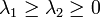 ) and the corresponding eigenvectors
  summarize the distribution of the gradient of within the window defined by
  centered at
  .[1][2][3]
Namely, if  , then
  (or
(or  ) is the direction that is maximally aligned with the gradient within the window. In particular, if
  then the gradient is always a multiple of (positive, negative or zero); this is the case if and only if within the window varies along the direction but is constant along
  .
.
If  , on the other hand, the gradient in the window has no predominant direction; which happens, for instance, when the image has rotational symmetry within that window. In particular,
  if and only if the function is constant (
 ) within
  .
.
More generally, the value of  , for k=1 or k=2, is the -weighted average, in the neighborhood of p, of the square of the directional derivative of along
  . The relative discrepancy between the two eigenvalues of is an indicator of the degree of anisotropy of the gradient in the window, namely how strongly is it biased towards a particular direction (and its opposite).[4][5] This attribute can be quantified by the coherence, defined as
if  . This quantity is 1 when the gradient is totally aligned, and 0 when it has no preferred direction. The formula is undefined, even in the limit, when the image is constant in the window (). Some authors define it as 0 in that case.
Note that the average of the gradient  inside the window is not a good indicator of anisotropy. Aligned but oppositely oriented gradient vectors would cancel out in this average, whereas in the structure tensor they are properly added together.[6]
By expanding the effective radius of the window function (that is, increasing its variance), one can make the structure tensor more robust in the face of noise, at the cost of diminished spatial resolution.[5][7] The formal basis for this property is described in more detail below, where it is shown that a multi-scale formulation of the structure tensor, referred to as the multi-scale structure tensor, constitutes a true multi-scale representation of directional data under variations of the spatial extent of the window function.
The 3D structure tensor
Definition
The structure tensor can be defined also for a function of three variables p=(x,y,z) in an entirely analogous way. Namely, in the continuous version we have , where
![S_0(p) =
\begin{bmatrix}
(I_x(p))^2 & I_x(p)I_y(p) & I_x(p)I_z(p) \\[10pt]
I_x(p)I_y(p) & (I_y(p))^2 & I_y(p)I_z(p) \\[10pt]
I_x(p)I_z(p) & I_y(p)I_z(p) & (I_z(p))^2
\end{bmatrix}](../I/m/bcfc0d5349b493adad578efcca4a2433.png)
where  are the three partial derivatives of , and the integral ranges over
  .
.
In the discrete version,, where
![S_0[p] =
\begin{bmatrix}
(I_x[p])^2 & I_x[p]I_y[p] & I_x[p]I_z[p] \\[10pt]
I_x[p]I_y[p] & (I_y[p])^2 & I_y[p]I_z[p]\\[10pt]
I_x[p]I_z[p] & I_y[p]I_z[p] & (I_z[p])^2
\end{bmatrix}](../I/m/22d076fe17b6953bf900f4e422609c76.png)
and the sum ranges over a finite set of 3D indices, usually  for some m.
Interpretation
As in the two-dimensional case, the eigenvalues  of
of ![S_w[p]](../I/m/609cc2abb432bc1b3c7ea35b7b6a43cc.png) , and the corresponding eigenvectors
, and the corresponding eigenvectors  , summarize the distribution of gradient directions within the neighborhood of p defined by the window . This information can be visualized as an ellipsoid whose semi-axes are equal to the eigenvalues and directed along their corresponding eigenvectors.[8]

In particular, if the ellipsoid is stretched along one axis only, like a cigar (that is, if  is much larger than both
  and
and  ), it means that the gradient in the window is predominantly aligned with the direction , so that the isosurfaces of tend to be flat and perpendicular to that vector. This situation occurs, for instance, when p lies on a thin plate-like feature, or on the smooth boundary between two regions with contrasting values.
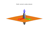 The structure tensor ellipsoid of a surface-like neighborhood ("surfel"), where  . . | 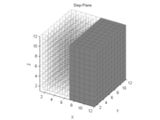 A 3D window straddling a smooth boundary surface between two uniform regions of a 3D image. |  The corresponding structure tensor ellipsoid. |
If the ellipsoid is flattened in one direction only, like a pancake (that is, if is much smaller than both and ), it means that the gradient directions are spread out but perpendicular to  ; so that the isosurfaces tend to be like tubes parallel to that vector. This situation occurs, for instance, when p lies on a thin line-like feature, or on a sharp corner of the boundary between two regions with contrasting values.
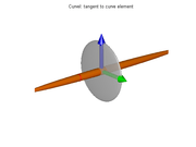 The structure tensor of a line-like neighborhood ("curvel"), where  . . |  A 3D window straddling a line-like feature of a 3D image. |  The corresponding structure tensor ellipsoid. |
Finally, if the ellipsoid is roughly spherical (that is, if  ), it means that the gradient directions in the window are more or less evenly distributed, with no marked preference; so that the function is mostly isotropic in that neighborhood. This happens, for instance, when the function has spherical symmetry in the neighborhood of p. In particular, if the ellipsoid degenerates to a point (that is, if the three eigenvalues are zero), it means that is constant (has zero gradient) within the window.
 The structure tensor in an isotropic neighborhood, where . | 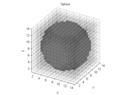 A 3D window containing a spherical feature of a 3D image. | 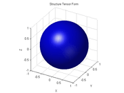 The corresponding structure tensor ellipsoid. |
The multi-scale structure tensor
The structure tensor is an important tool in scale space analysis. The multi-scale structure tensor (or multi-scale second moment matrix) of a function is in contrast to other one-parameter scale-space features an image descriptor that is defined over two scale parameters.
One scale parameter, referred to as local scale  , is needed for determining the amount of pre-smoothing when computing the image gradient
  . Another scale parameter, referred to as integration scale
  , is needed for specifying the spatial extent of the window function
  that determines the weights for the region in space over which the components of the outer product of the gradient by itself
  are accumulated.
More precisely, suppose that is a real-valued signal defined over  . For any local scale
  , let a multi-scale representation
  of this signal be given by
  where
where  represents a pre-smoothing kernel. Furthermore, let denote the gradient of the scale space representation.
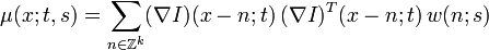
Then, the multi-scale structure tensor/second-moment matrix is defined by
[7][9][10]
represents a pre-smoothing kernel. Furthermore, let denote the gradient of the scale space representation.
Then, the multi-scale structure tensor/second-moment matrix is defined by
[7][9][10]
Conceptually, one may ask if it would be sufficient to use any self-similar families of smoothing functions and . If one naively would apply, for example, a box filter, however, then non-desirable artifacts could easily occur. If one wants the multi-scale structure tensor to be well-behaved over both increasing local scales and increasing integration scales , then it can be shown that both the smoothing function and the window function have to be Gaussian.[7] The conditions that specify this uniqueness are similar to the scale-space axioms that are used for deriving the uniqueness of the Gaussian kernel for a regular Gaussian scale space of image intensities.
There are different ways of handling the two-parameter scale variations in this family of image descriptors. If we keep the local scale parameter fixed and apply increasingly broadened versions of the window function by increasing the integration scale parameter only, then we obtain a true formal scale space representation of the directional data computed at the given local scale .[7] If we couple the local scale and integration scale by a relative integration scale  , such that
  then for any fixed value of
  , we obtain a reduced self-similar one-parameter variation, which is frequently used to simplify computational algorithms, for example in corner detection, interest point detection, texture analysis and image matching.
By varying the relative integration scale in such a self-similar scale variation, we obtain another alternative way of parameterizing the multi-scale nature of directional data obtained by increasing the integration scale.
, we obtain a reduced self-similar one-parameter variation, which is frequently used to simplify computational algorithms, for example in corner detection, interest point detection, texture analysis and image matching.
By varying the relative integration scale in such a self-similar scale variation, we obtain another alternative way of parameterizing the multi-scale nature of directional data obtained by increasing the integration scale.
A conceptually similar construction can be performed for discrete signals, with the convolution integral replaced by a convolution sum and with the continuous Gaussian kernel  replaced by the discrete Gaussian kernel
  :
:
When quantizing the scale parameters and in an actual implementation, a finite geometric progression  is usually used, with i ranging from 0 to some maximum scale index m. Thus, the discrete scale levels will bear certain similarities to image pyramid, although spatial subsampling may not necessarily be used in order to preserve more accurate data for subsequent processing stages.
Applications
The eigenvalues of the structure tensor play a significant role in many image processing algorithms, for problems like corner detection, interest point detection, and feature tracking.[8][11][12][13][14][15][16] The structure tensor also plays a central role in the Lucas-Kanade optical flow algorithm, and in its extensions to estimate affine shape adaptation;[9] where the magnitude of is an indicator of the reliability of the computed result. The tensor has also been used for scale space analysis,[7] estimation of local surface orientation from monocular or binocular cues,[10] non-linear fingerprint enhancement,[17] diffusion-based image processing,[18][19][20][21] and several other image processing problems.
Processing spatio-temporal video data with the structure tensor
The three-dimensional structure tensor has been used to analyze three-dimensional video data (viewed as a function of x, y, and time t).[4]
If one in this context aims at image descriptors that are invariant under Galilean transformations, to make it possible to compare image measurements that have been obtained under variations of a priori unknown image velocities 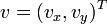
 ,
,
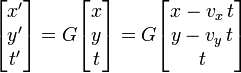
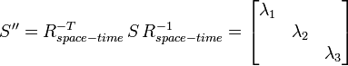
it is, however, from a computational viewpoint more preferable to parameterize the components in the structure tensor/second-moment matrix  using the notion of Galilean diagonalization[22]
where  denotes a Galilean transformation of space-time and
  a two-dimensional rotation over the spatial domain,
compared to the abovementioned use of eigenvalues of a 3-D structure tensor, which corresponds to an eigenvalue decomposition and a (non-physical) three-dimensional rotation of space-time
a two-dimensional rotation over the spatial domain,
compared to the abovementioned use of eigenvalues of a 3-D structure tensor, which corresponds to an eigenvalue decomposition and a (non-physical) three-dimensional rotation of space-time
 .
.
To obtain true Galilean invariance, however, also the shape of the spatio-temporal window function needs to be adapted,[22][23] corresponding to the transfer of affine shape adaptation[9] from spatial to spatio-temporal image data. In combination with local spatio-temporal histogram descriptors,[24] these concepts together allow for Galilean invariant recognition of spatio-temporal events.[25]
See also
- Tensor
- Tensor operator
- Directional derivative
- Gaussian
- Corner detection
- Edge detection
- Lucas-Kanade method
- Affine shape adaptation
References
- ↑ 1.0 1.1 J. Bigun and G. Granlund (1986), Optimal Orientation Detection of Linear Symmetry. Tech. Report LiTH-ISY-I-0828, Computer Vision Laboratory, Linkoping University, Sweden 1986; Thesis Report, Linkoping studies in science and technology No. 85, 1986.
- ↑ 2.0 2.1 J. Bigun and G. Granlund (1987). "Optimal Orientation Detection of Linear Symmetry". First int. Conf. on Computer Vision, ICCV, (London). Piscataway: IEEE Computer Society Press, Piscataway. pp. 433–438.
- ↑ 3.0 3.1 H. Knutsson (1989). "Representing local structure using tensors". Proceedings 6th Scandinavian Conf. on Image Analysis. Oulu: Oulu University. pp. 244–251.
- ↑ 4.0 4.1 B. Jahne (1993). Spatio-Temporal Image Processing: Theory and Scientific Applications 751. Berlin: Springer-Verlag.
- ↑ 5.0 5.1 G. Medioni, M. Lee and C. Tang (March 2000). A Computational Framework for Feature Extraction and Segmentation. Elsevier Science.
- ↑ T. Brox, J. Weickert, B. Burgeth and P. Mrazek (2004). "Nonlinear Structure Tensors" (113). pp. 1–32.
- ↑ 7.0 7.1 7.2 7.3 7.4 T. Lindeberg (1994), Scale-Space Theory in Computer Vision. Kluwer Academic Publishers, (see sections 14.4.1 and 14.2.3 on pages 359-360 and 355-356 for detailed statements about how the multi-scale second-moment matrix/structure tensor defines a true and uniquely determined multi-scale representation of directional data).
- ↑ 8.0 8.1 M. Nicolescu and G. Medioni (2003). "Motion Segmentation with Accurate Boundaries — A Tensor Voting Approach". Proc. IEEE Computer Vision and Pattern Recognition 1. pp. 382–389.
- ↑ 9.0 9.1 9.2 T. Lindeberg and J. Garding (1997). "Shape-adapted smoothing in estimation of 3-D depth cues from affine distortions of local 2-D structure". Image and Vision Computing 15 (6): pp 415–434. doi:10.1016/S0262-8856(97)01144-X.
- ↑ 10.0 10.1 J. Garding and T. Lindeberg (1996). "Direct computation of shape cues using scale-adapted spatial derivative operators, International Journal of Computer Vision, volume 17, issue 2, pages 163--191.
- ↑ W. Förstner (1986). "A Feature Based Correspondence Algorithm for Image Processing" 26. pp. 150–166.
- ↑ C. Harris and M. Stephens (1988). "A Combined Corner and Edge Detector". Proc. of the 4th ALVEY Vision Conference. pp. 147–151.
- ↑ K. Rohr (1997). "On 3D Differential Operators for Detecting Point Landmarks" 15 (3). pp. 219–233.
- ↑ I. Laptev and T. Lindeberg (2003). "Space-time interest points". International Conference on Computer Vision ICCV'03 I. pp. 432–439. doi:10.1109/ICCV.2003.1238378.
- ↑ B. Triggs (2004). "Detecting Keypoints with Stable Position, Orientation, and Scale under Illumination Changes". Proc. European Conference on Computer Vision 4. pp. 100–113.
- ↑ C. Kenney, M. Zuliani and B. Manjunath, (2005). "An Axiomatic Approach to Corner Detection". Proc. IEEE Computer Vision and Pattern Recognition. pp. 191–197.
- ↑ A. Almansa and T. Lindeberg (2000), Enhancement of fingerprint images using shape-adaptated scale-space operators. IEEE Transactions on Image Processing, volume 9, number 12, pages 2027-2042.
- ↑ J. Weickert (1998), Anisotropic diffusion in image processing, Teuber Verlag, Stuttgart.
- ↑ D. Tschumperle and Deriche (September 2002). "Diffusion PDE's on Vector-Valued Images". pp. 16–25.
- ↑ S. Arseneau and J. Cooperstock (September 2006). "An Asymmetrical Diffusion Framework for Junction Analysis". British Machine Vision Conference 2. pp. 689–698.
- ↑ S. Arseneau, and J. Cooperstock (November 2006). "An Improved Representation of Junctions through Asymmetric Tensor Diffusion". International Symposium on Visual Computing.
- ↑ 22.0 22.1 T. Lindeberg, A. Akbarzadeh, and I. Laptev (August 2004). "Galilean-corrected spatio-temporal interest operators". International Conference on Pattern Recognition ICPR'04 I. pp. 57–62. doi:10.1109/ICPR.2004.1334004.
- ↑ I. Laptev, and T. Lindeberg (August 2004). "Velocity adaptation of space-time interest points". International Conference on Pattern Recognition ICPR'04 I. pp. 52–56. doi:10.1109/ICPR.2004.971.
- ↑ I. Laptev, and T. Lindeberg (May 2004). "Local descriptors for spatio-temporal recognition". ECCV'04 Workshop on Spatial Coherence for Visual Motion Analysis (Prague, Czech Republic) Springer Lecture Notes in Computer Science 3667. pp. 91–103. doi:10.1007/11676959.
- ↑ I. Laptev, B. Caputo, C. Schuldt, and T. Lindeberg (2007). "Local velocity-adapted motion events for spatio-temporal recognition". Computer Vision and Image Understanding 108. pp. 207–229. doi:10.1016/j.cviu.2006.11.023.