Stokes phenomenon

In complex analysis the Stokes phenomenon, discovered by G. G. Stokes (1847, 1858), is that the asymptotic behavior of functions can differ in different regions of the complex plane. These regions are bounded by Stokes line or anti-Stokes lines.

Stokes lines and anti-Stokes lines

Somewhat confusingly, mathematicians and physicists use the terms "Stokes line" and "anti-Stokes line" in opposite ways. The lines originally studied by Stokes are what some mathematicians call anti-Stokes lines and what physicists call Stokes lines. (These terms are also used in optics for the unrelated Stokes lines and antiStokes lines in Raman scattering). This article uses the physicist's convention, which is historically more accurate and seems to be becoming more common among mathematicians. Olver (1997) recommends the term "principal curve" for (physicist's) anti-Stokes lines.

Informally the antiStokes lines are roughly where some term in the asymptotic expansion changes from increasing to decreasing, and the Stokes lines are lines along which some term approaches infinity or zero fastest. AntiStokes lines bound regions where the function has some asymptotic behavior. The Stokes lines and antiStokes lines are not unique and do not really have a precise definition in general, because the region where a function has a given asymptotic behavior is a somewhat vague concept. However the lines do usually have well determined directions at essential singularities of the function, and there is sometimes a natural choice of these lines as follows. The asymptotic expansion of a function is often give by a linear combination of functions of the form f(z)e^±g(z) for functions f and g. The Stokes lines can then be taken as the zeros of the imaginary part of g, and the antiStokes lines as the zeros of the real part of g. (This is not quite canonical, because one can add a constant to g, changing the lines.) If the lines are defined like this then they are orthogonal where they meet, unless g has a multiple zero.

As a trivial example, the function sinh(z) has two regions Re(z)>0 and Re(z)<0 where it is asymptotic to e^z/2 and e^−z/2. So the antiStokes line can be taken to be the imaginary axis, and the Stokes line can be taken to be the real axis. One could equally well take the Stokes line to be any line of given imaginary part; these choices differ only by change of variables, showing that there is no canonical choice for the Stokes line.

Example: the Airy function

The Airy function Ai(x) is one of two solutions to a simple differential equation

y'' - xy = 0 , \,

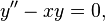
which it is often useful to approximate for many values of x – including complex values. For large x of given argument the solution can be approximated by a linear combination of the functions

\frac{e^{\pm\frac23x^{3/2}}}{x^{1/4}}.

However the linear combination has to change as the argument of x passes certain values because these approximations are mutli-valued functions but the Airy function is single valued. For example, if we regard the limit of x as large and real, and would like to approximate the Airy function for both positive and negative values, we would find that

Plot of Ai(x) in red and Bi(x) in blue

\begin{align} \mathrm{Ai}(x) &{}\sim \frac{e^{-\frac23x^{3/2}}}{2\sqrt\pi\,x^{1/4}} \\ \mathrm{Ai}(-x) &{}\sim \frac{\sin(\frac23x^{3/2}+\frac14\pi)}{\sqrt\pi\,x^{1/4}} \\ \end{align}

Stokes lines and antiStokes lines for the Airy function

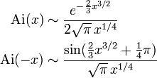
which are two very different expressions. What has happened is that as we have increased the argument of x from 0 to pi (rotating it around through the upper half complex plane) we have crossed an antiStokes line, which in this case is at 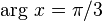$\operatorname{arg}\, x = \pi / 3$ . At this antiStokes line, the coefficient of $\frac{e^{-\frac23x^{3/2}}}{x^{1/4}}$ is forced to jump. The coefficient of $\frac{e^{+\frac23x^{3/2}}}{x^{1/4}}$ can jump at this line but is not forced to; it can change gradually as arg x varies from π/3 to π as it is not determined in this region.

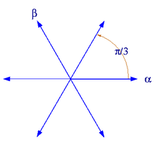
There are three antiStokes lines with arguments π/3, π. –π/3, and three Stokes lines with arguments 2π/3, 0. –2π/3.

Example: second order linear differential equations

The Airy function example can be generalized to solutions of second order linear differential equations as follows. By standard changes of variables the equation can usually be changed to one of the form

\frac{d^2w}{dz^2} = f(z)w

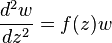
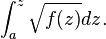
where f is holomorphic in a simply connected region and w is a solution of the differential equation. Then in some cases w has an asymptotic approximation as a linear combination of functions of the form

\frac{\exp{\pm\int_{a}^z\sqrt{f(z)}dz}}{f(z)^{1/4}}

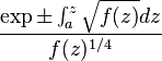
for some constant a, and the antiStokes lines and Stokes lines can be taken as the zeros of the real and imaginary parts of

\int_{a}^z\sqrt{f(z)}dz.

If a is a simple zero of f there are three Stokes lines and three anti-Stokes lines meeting, as in the case of the Airy function where f(z)=z has a simple zero at z=0.

References

Berry, M. V. (1988), "Stokes' phenomenon; smoothing a Victorian discontinuity.", Inst. Hautes Études Sci. Publ. Math. 68: 211–221, doi:10.1007/bf02698550, MR 1001456
Berry, M. V. (1989), "Uniform asymptotic smoothing of Stokes's discontinuities", Proc. Roy. Soc. London Ser. A 422 (1862): 7–21, doi:10.1098/rspa.1989.0018, JSTOR 2398522, MR 0990851
Meyer, R. E. (1989), "A simple explanation of the Stokes phenomenon", SIAM Rev. 31 (3): 435–445, doi:10.1137/1031090, JSTOR 2031404, MR 1012299
Olver, Frank W. J. (1997) [1974], Asymptotics and special functions, AKP Classics, Wellesley, MA: A K Peters Ltd., ISBN 978-1-56881-069-0, MR 1429619
Stokes, G. G. (1847), "On the numerical calculation of a class of definite integrals and infinite series", Transactions of the Cambridge philosophical society IX (I): 166–189
Stokes, G. G. (1858), "On the discontinuity of arbitrary constants which appear in divergent developments", Transactions of the Cambridge philosophical society X (I): 105–128

Witten, Ed (2010). "Analytic Continuation Of Chern-Simons Theory". v4. arXiv:hep-th/1001.2933 Check |arxiv= value (help).