Stochastic gradient descent

Stochastic gradient descent is a gradient descent optimization method for minimizing an objective function that is written as a sum of differentiable functions.

Background

Both statistical estimation and machine learning consider the problem of minimizing an objective function that has the form of a sum:

Q(w) = \sum_{i=1}^n Q_i(w),

where the parameter $w$ is to be estimated and where typically each summand function $Q_i$ is associated with the $i$ -th observation in the data set (used for training).

In classical statistics, sum-minimization problems arise in least squares and in maximum-likelihood estimation (for independent observations). The general class of estimators that arise as minimizers of sums are called M-estimators. However, in statistics, it has been long recognized that requiring even local minimization is too restrictive for some problems of maximum-likelihood estimation, as shown for example by Thomas Ferguson's example.^[1] Therefore, contemporary statistical theorists often consider stationary points of the likelihood function (or zeros of its derivative, the score function, and other estimating equations).

The sum-minimization problem also arises for empirical risk minimization: In this case, $Q_i(w)$ is the value of the loss function at $i$ -th example, and $Q(w)$ is the empirical risk.

When used to minimize the above function, a standard (or "batch") gradient descent method would perform the following iterations :

w := w - \alpha \nabla Q(w) = w - \alpha \sum_{i=1}^n \nabla Q_i(w),

where $\alpha$ is a step size (sometimes called the learning rate in machine learning).

In many cases, the summand functions have a simple form that enables inexpensive evaluations of the sum-function and the sum gradient. For example, in statistics, one-parameter exponential families allow economical function-evaluations and gradient-evaluations.

However, in other cases, evaluating the sum-gradient may require expensive evaluations of the gradients from all summand functions. When the training set is enormous and no simple formulas exist, evaluating the sums of gradients becomes very expensive, because evaluating the gradient requires evaluating all the summand functions' gradients. To economize on the computational cost at every iteration, stochastic gradient descent samples a subset of summand functions at every step. This is very effective in the case of large-scale machine learning problems.^[2]

Iterative method

Fluctuations in the total objective function as gradient steps with respect to mini-batches are taken.

In stochastic (or "on-line") gradient descent, the true gradient of $Q(w)$ is approximated by a gradient at a single example:

w := w - \alpha \nabla Q_i(w).

As the algorithm sweeps through the training set, it performs the above update for each training example. Several passes can be made over the training set until the algorithm converges. If this is done, the data can be shuffled for each pass to prevent cycles. Typical implementations may use an adaptive learning rate so that the algorithm converges.

In pseudocode, stochastic gradient descent can be presented as follows:

Choose an initial vector of parameters $w$ and learning rate $\alpha$ .
Randomly shuffle examples in the training set.
Repeat until an approximate minimum is obtained:
- For , do:
  - $\! w := w - \alpha \nabla Q_i(w).$

A compromise between the two forms called "mini-batches" computes the gradient against more than one training examples at each step. This can perform significantly better than true stochastic gradient descent because the code can make use of vectorization libraries rather than computing each step separately. It may also result in smoother convergence, as the gradient computed at each step uses more training examples.

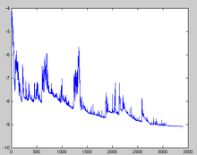
The convergence of stochastic gradient descent has been analyzed using the theories of convex minimization and of stochastic approximation. Briefly, when the learning rates $\alpha$ decrease with an appropriate rate, and subject to relatively mild assumptions, stochastic gradient descent converges almost surely to a global minimum when the objective function is convex or pseudoconvex, and otherwise converges almost surely to a local minimum.^[3] ^[4] This is in fact a consequence of the Robbins-Siegmund theorem.^[5]

Example

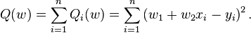
Let's suppose we want to fit a straight line $y = \! w_1 + w_2 x$ to a training set of two-dimensional points $\! (x_1, y_1), \ldots, (x_n, y_n)$ using least squares. The objective function to be minimized is:

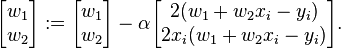
Q(w) = \sum_{i=1}^n Q_i(w) = \sum_{i=1}^n \left(w_1 + w_2 x_i - y_i\right)^2.

The last line in the above pseudocode for this specific problem will become:

\begin{bmatrix} w_1 \\ w_2 \end{bmatrix} := \begin{bmatrix} w_1 \\ w_2 \end{bmatrix} - \alpha \begin{bmatrix} 2 (w_1 + w_2 x_i - y_i) \\ 2 x_i(w_1 + w_2 x_i - y_i) \end{bmatrix}.

Applications

Stochastic gradient descent is a popular algorithm for training a wide range of models in machine learning, including (linear) support vector machines, logistic regression (see, e.g., Vowpal Wabbit) and graphical models.^[6] It competes with the L-BFGS algorithm,^[7] which is also widely used. SGD has been used since at least 1960 for training linear regression models, originally under the name ADALINE.^[8]

When combined with the backpropagation algorithm, it is the de facto standard algorithm for training artificial neural networks.

Another popular stochastic gradient descent algorithm is the least mean squares (LMS) adaptive filter.

References

↑ Ferguson, Thomas S. (1982). "An inconsistent maximum likelihood estimate". Journal of the American Statistical Association 77 (380): 831–834. doi:10.1080/01621459.1982.10477894. JSTOR 2287314.
↑ Bottou, Léon; Bousquet, Olivier (2008). The Tradeoffs of Large Scale Learning. Advances in Neural Information Processing Systems 20. pp. 161–168.
↑ Bottou, Léon (1998). "Online Algorithms and Stochastic Approximations". Online Learning and Neural Networks. Cambridge University Press. ISBN 978-0-521-65263-6
↑ Kiwiel, Krzysztof C. (2001). "Convergence and efficiency of subgradient methods for quasiconvex minimization". Mathematical Programming (Series A) 90 (1) (Berlin, Heidelberg: Springer). pp. 1–25. doi:10.1007/PL00011414. ISSN 0025-5610. MR 1819784.
↑ Robbins, Herbert; Siegmund, David O. (1971). "A convergence theorem for non negative almost supermartingales and some applications". In Rustagi, Jagdish S. Optimizing Methods in Statistics. Academic Press
↑ Jenny Rose Finkel, Alex Kleeman, Christopher D. Manning (2008). Efficient, Feature-based, Conditional Random Field Parsing. Proc. Annual Meeting of the ACL.
↑ Citation Needed
↑ Avi Pfeffer. "CS181 Lecture 5 — Perceptrons". Harvard University.

Recommended Literature

Bertsekas, Dimitri (2003). Convex Analysis and Optimization. Athena Scientific.

Bertsekas, Dimitri P. (1999). Nonlinear Programming (Second ed.). Cambridge, MA.: Athena Scientific. ISBN 1-886529-00-0.

Bottou, Léon (2004). "Stochastic Learning". Advanced Lectures on Machine Learning. LNAI 3176, Springer Verlag. pp. 146–168. ISBN 978-3-540-23122-6

Davidon, W. C. (1976). "New least-square algorithms". Journal of Optimization Theory and Applications 18 (2). pp. 187–197. doi:10.1007/BF00935703. MR 418461.

Kiwiel, Krzysztof C. (2003). "Convergence of approximate and incremental subgradient methods for convex optimization". SIAM Journal of Optimization 14 (3). pp. 807–840. doi:10.1137/S1052623400376366. MR 2085944. (Extensive list of references)

Pattern Classification by Richard O. Duda, Peter E. Hart, David G. Stork, ISBN 0-471-05669-3, 2000

Introduction to Stochastic Search and Optimization by James C. Spall, ISBN 0-471-33052-3, 2003

Software

sgd: an LGPL C++ library which uses stochastic gradient descent to fit SVM and conditional random field models.
CRF-ADF A C# toolkit of stochastic gradient descent and its feature-frequency-adaptive variation for training conditional random field models.

External links

Using stochastic gradient descent in C++, Boost, Ublas for linear regression