Stieltjes constants
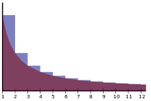
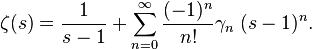
In mathematics, the Stieltjes constants are the numbers  that occur in the Laurent series expansion of the Riemann zeta function:
The zero'th constant  is known as the Euler–Mascheroni constant.
Representations
The Stieltjes constants are given by the limit
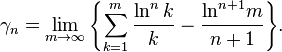
(In the case n = 0, the first summand requires evaluation of 00, which is taken to be 1.)
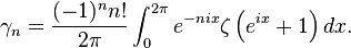
Cauchy's differentiation formula leads to the integral representation
Various representations in terms of integrals and infinite series are given in works of Jensen, Franel, Hermite, Hardy, Ramanujan, Ainsworth, Howell, Coppo, Connon, Coffey, Choi, Blagouchine and some other authors.[1][2][3][4][5][6] In particular, Jensen-Franel's integral formula, often erroneously attributed to Ainsworth and Howell, states that

where δn,k is the Kronecker symbol (Kronecker delta).[5][6] Among other formulae, we find

![\begin{array}{l}
\displaystyle
\gamma_1 =-\left[\gamma -\frac{\ln2}{2}\right]\ln2+\,i\!\int\limits_0^\infty \! \frac{dx}{e^{\pi x}+1} \left\{
\frac{\ln(1-ix)}{1-ix} - \frac{\ln(1+ix)}{1+ix}
\right\}\, \\[6mm]
\displaystyle
\gamma_1 = -\gamma^2 - \int\limits_0^\infty \left[\frac{1}{1-e^{-x}}-\frac{1}{x}\right] e^{-x}\ln x \, dx
\end{array}](../I/m/3a2c8189ca0ccf36c4d00fc0c0ba1001.png)
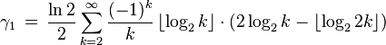
As concerns series representations, a famous series implying an integer part of a logarithm was given by Hardy in 1912[8]
Israilov[9] gave semi-convergent series in terms of Bernoulli numbers 
![\gamma_m\,=\,\sum_{k=1}^n \frac{\,\ln^m\! k\,}{k} - \frac{\,\ln^{m+1}\! n\,}{m+1}
- \frac{\,\ln^m\! n\,}{2n} - \sum_{k=1}^{N-1} \frac{\,B_{2k}\,}{(2k)!}\left[\frac{\ln^m\! x}{x}\right]^{(2k-1)}_{x=n}
+ \theta\cdot\frac{\,B_{2N}\,}{(2N)!}\left[\frac{\ln^m\! x}{x}\right]^{(2N-1)}_{x=n} \,,\qquad 0<\theta<1](../I/m/f7cf7577b8eb83458bafa99dc00e94d4.png)
Oloa and Tauraso[10] showed that series with harmonic numbers may lead to Stieltjes constants
![\begin{array}{l}
\displaystyle
\sum_{n=1}^\infty \frac{\,H_n - (\gamma+\ln n)\,}{n} \,=\,
\,-\gamma_1 -\frac{1}{2}\gamma^2+\frac{1}{12}\pi^2 \\[6mm]
\displaystyle
\sum_{n=1}^\infty \frac{\,H^{(2)}_n - (\gamma+\ln n)^2\,}{n} \,=\,
\,-\gamma_2 -2\gamma\gamma_1 -\frac{2}{3}\gamma^3+\frac{5}{3}\zeta(3)
\end{array}](../I/m/08067b1238ec1902cd638161fd22f860.png)
Blagouchine[6] obtained slowly-convergent series involving unsigned Stirling numbers of the first kind
![\left[{\cdot \atop \cdot}\right]](../I/m/365a328c78f928ffc81ab92543234b78.png)
![\gamma_m\,=\,\frac{1}{2}\delta_{m,0}+
\frac{\,(-1)^m m!\,}{\pi} \sum_{n=1}^\infty\frac{1}{\,n\cdot n!\,}
\sum_{k=0}^{\lfloor\!\frac{1}{2}n\!\rfloor}\frac{\,(-1)^{k}\cdot\left[{2k+2\atop m+1}\right] \cdot\left[{n\atop 2k+1}\right]\,}
{\,(2\pi)^{2k+1}\,}\,,\qquad m=0,1,2,...,](../I/m/953272cfb85a015cc553d62d282a867f.png)
as well as semi-convergent series with rational terms only
![\gamma_m\,
=\,\frac{1}{2}\delta_{m,0}+(-1)^{m} m!\cdot\!\sum_{k=1}^{N}\frac{\,\left[{2k\atop m+1}\right]\cdot B_{2k}\,}{(2k)!}
\,+\, \theta\cdot\frac{\,(-1)^{m} m!\!\cdot \left[{2N+2\atop m+1}\right]\cdot B_{2N+2}\,}{(2N+2)!}\,,\qquad 0<\theta<1](../I/m/e105baf4a73b408e3cef760835797fe9.png)
where m=0,1,2,... Several other series are given in works of Coffey.[2][3]
Asymptotic growth
The Stieltjes constants satisfy the bound
![\big|\gamma_n\big|\,\leqslant\,
\begin{cases}
\displaystyle \frac{2\,(n-1)!}{\pi^n}\,,\qquad & n=1, 3, 5,\ldots \\[3mm]
\displaystyle \frac{4\,(n-1)!}{\pi^n}\,,\qquad & n=2, 4, 6,\ldots
\end{cases}](../I/m/66b75041e476e38ea34dc5de283b69ca.png)
given by Berndt in 1972.[11] Better bounds were obtained by Lavrik, Israilov, Matsuoka, Nan-You, Williams, Knessl, Coffey, Adell, Saad-Eddin, Fekih-Ahmed and Blagouchine (see the list of references given in[6]). One of the best estimations, in terms of elementary functions, belongs to Matsuoka:

As concerns estimations resorting to non-elementary functions, Knessl, Coffey[12] and Fekih-Ahmed[13] obtained quite accurate results. For example, Knessl and Coffey give the following formula that approximates the Stieltjes constants relatively well for large n.[12] If v is the unique solution of
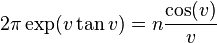
with 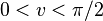 , and if
  , then
where
![B = \frac{2 \sqrt{2\pi} \sqrt{u^2+v^2}}{[(u+1)^2+v^2]^{1/4}}](../I/m/20cb691f31babf736862c4f85ef3d794.png)
Up to n = 100000, the Knessl-Coffey approximation correctly predicts the sign of γn with the single exception of n = 137.[12]
Numerical values
The first few values are:
n approximate value of γn OEIS 0 +0.5772156649015328606065120900824024310421593359 A001620 1 −0.0728158454836767248605863758749013191377363383 A082633 2 −0.0096903631928723184845303860352125293590658061 A086279 3 +0.0020538344203033458661600465427533842857158044 A086280 4 +0.0023253700654673000574681701775260680009044694 A086281 5 +0.0007933238173010627017533348774444448307315394 A086282 6 −0.0002387693454301996098724218419080042777837151 A183141 7 −0.0005272895670577510460740975054788582819962534 A183167 8 −0.0003521233538030395096020521650012087417291805 A183206 9 −0.0000343947744180880481779146237982273906207895 A184853 10 +0.0002053328149090647946837222892370653029598537 A184854 100 −4.2534015717080269623144385197278358247028931053 × 10¹⁷ 1000 −1.5709538442047449345494023425120825242380299554 × 10486 10000 −2.2104970567221060862971082857536501900234397174 × 106883 100000 +1.9919273063125410956582272431568589205211659777 × 1083432
For large n, the Stieltjes constants grow rapidly in absolute value, and change signs in a complex pattern.
Further information related to the numerical evaluation of Stieltjes constants may be found in works of Keiper,[14] Kreminski,[15] Plouffe[16] and Johansson.[17] The latter author provided values of the Stieltjes constants up to n = 100000, accurate to over 10000 digits each. The numerical values can be retrieved from the LMFDB .
Generalized Stieltjes constants
General information
More generally, one can define Stieltjes constants γn(a) that occur in the Laurent series expansion of the Hurwitz zeta function:
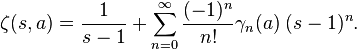
Here a is a complex number with Re(a)>0. Since the Hurwitz zeta function is a generalization of the Riemann zeta function, we have γn(1)=γn The zero'th constant is simply the digamma-function γ0(a)=-Ψ(a),[18] while other constants are not known to be reducible to any elementary or classical function of analysis. Nevertheless, there are numeorous representations for them. For example, there exists the following asymptotic representation
![\gamma_n(a) \,=\, \lim_{m\to\infty}\left\{
\sum_{k=0}^m \frac{\ln^n (k+a)}{k+a} - \frac{\ln^{n+1} (m+a)}{n+1}
\right\}\,, \qquad\;
\begin{array}{l}
n=0, 1, 2,\ldots\, \\[1mm]
a\neq0, -1, -2, \ldots
\end{array}](../I/m/af9321202b0d71dc27d29846857fc013.png)
due to Berndt and Wilton. The analog of Jensen-Franel's formula for the generalized Stieltjes constant is the Hermite formula[5]
![\gamma_n(a) \,=\,\left[\frac{1}{2a}-\frac{\ln{a}}{n+1} \right]\ln^n\!{a}
-i\!\int\limits_0^\infty \! \frac{dx}{e^{2\pi x}-1} \left\{
\frac{\ln^n(a-ix)}{a-ix} - \frac{\ln^n(a+ix)}{a+ix}
\right\} \,, \qquad\;
\begin{array}{l}
n=0, 1, 2,\ldots\, \\[1mm]
a\neq0, -1, -2, \ldots
\end{array}](../I/m/c931a86e871fcdbf2640d86b66379bee.png)
Generalized Stieltjes constants satisfy the following recurrent relationship
![\gamma_n(a+1) \, =\, \gamma_n(a) - \frac{\,\ln^n\! a\,}{a}
\,, \qquad\;
\begin{array}{l}
n=0, 1, 2,\ldots\, \\[1mm]
a\neq0, -1, -2, \ldots
\end{array}](../I/m/e1bc2ed224ab95ef4dd17071dfa0ae1e.png)
as well as the multiplication theorem
![\sum_{l=0}^{n-1} \gamma_p\!\left(\! a+\frac{l}{\,n\,} \right) =\,
(-1)^p n \! \left[\frac{\ln n}{\,p+1\,} - \Psi(an) \right]\!\ln^p\! n \,+\, n\sum_{r=0}^{p-1}(-1)^r \binom{p}{r} \gamma_{p-r}(an) \cdot \ln^r\!{n}\,,
\qquad\qquad n=2, 3, 4,\ldots](../I/m/270b73a06bec501361e05f49988756e9.png)
where  denotes the binomial coefficient (see[19] and,[20] pp. 101–102).
First generalized Stieltjes constant
The first generalized Stieltjes constant has a number of remarkable properties.
- Malmsten's identity (reflection formula for the first generalized Stieltjes constants): the reflection formula for the first generalized Stieltjes constant has the following form

where m and n are positive integers such that m<n. This formula has been long-time attributed to Almkvist and Meurman who derived it in 1990s.[21] However, very recently Blagouchine found that this identity, albeit in a slightly different form, was first obtained by Carl Malmsten in 1846.[5][22]
- Rational arguments theorem: the first generalized Stieltjes constant at rational argument may be evaluated in a quasi closed-form via the following formula
![\begin{array}{ll}
\displaystyle
\gamma_1 \biggl(\frac{r}{m} \biggr)
=& \displaystyle
\gamma_1 +\gamma^2 + \gamma\ln2\pi m + \ln2\pi\cdot\ln{m}+\frac{1}{2}\ln^2\!{m}
+ (\gamma+\ln2\pi m)\cdot\Psi\!\left(\!\frac{r}{m}\!\right) \\[5mm]
\displaystyle & \displaystyle\qquad
+\pi\sum_{l=1}^{m-1} \sin\frac{2\pi r l}{m} \cdot\ln\Gamma \biggl(\frac{l}{m} \biggr)
+ \sum_{l=1}^{m-1} \cos\frac{2\pi rl}{m}\cdot\zeta''\!\left(\! 0,\,\frac{l}{m}\!\right)
\end{array}\,,\qquad\quad r=1, 2, 3,\ldots, m-1\,.](../I/m/f183d3d1632e8c21479d21763de04a6e.png)
due also to Blagouchine in.[5][18] An alternative proof was later proposed by Coffey.[23]
- Finite summations: there are numerous summation formulae for the first generalized Stieltjes constants. For example
![\begin{array}{ll}
\displaystyle
\sum_{r=0}^{m-1} \gamma_1\!\left(\! a+\frac{r}{\,m\,} \right) =\,
m\ln{m}\cdot\Psi(am) - \frac{m}{2}\ln^2\!m + m\gamma_1(am)\,,\qquad a\in\mathbb{C}\\[6mm]
\displaystyle
\sum_{r=1}^{m-1} \gamma_1\!\left(\!\frac{r}{\,m\,} \right) =\,
(m-1)\gamma_1 - m\gamma\ln{m} - \frac{m}{2}\ln^2\!m \\[6mm]
\displaystyle
\sum_{r=1}^{2m-1} (-1)^r \gamma_1 \biggl(\!\frac{r}{2m} \!\biggr)
\,=\, -\gamma_1+m(2\gamma+\ln2+2\ln m)\ln2\\[6mm]
\displaystyle
\sum_{r=0}^{2m-1} (-1)^r \gamma_1\biggl(\!\frac{2r+1}{4m} \!\biggr)
\,=\, m\left\{4\pi\ln\Gamma \biggl(\frac{1}{4} \biggr) - \pi\big(4\ln2+3\ln\pi+\ln m+\gamma \big)\!\right\}\\[6mm]
\displaystyle
\sum_{r=1}^{m-1} \gamma_1 \biggl(\!\frac{r}{m}\!\biggr)
\!\cdot\cos\dfrac{2\pi rk}{m} \,=\, -\gamma_1 + m(\gamma+\ln2\pi m)
\ln\!\left(\!2\sin\frac{\,k\pi\,}{m}\!\right)
+\frac{m}{2}
\left\{\zeta''\!\left(\! 0,\,\frac{k}{m}\!\right)+ \, \zeta''\!\left(\! 0,\,1-\frac{k}{m}\!\right) \! \right\}\,, \qquad k=1,2,\ldots,m-1 \\[6mm]
\displaystyle
\sum_{r=1}^{m-1} \gamma_1\biggl(\!\frac{r}{m} \!\biggr)
\!\cdot\sin\dfrac{2\pi rk}{m} \,=\,\frac{\pi}{2} (\gamma+\ln2\pi m)(2k-m)
- \frac{\pi m}{2} \left\{\ln\pi -\ln\sin\frac{k\pi}{m} \right\}
+ m\pi\ln\Gamma \biggl(\frac{k}{m} \biggr) \,, \qquad k=1,2,\ldots,m-1 \\[6mm]
\displaystyle
\sum_{r=1}^{m-1} \gamma_1 \biggl(\!\frac{r}{m} \!\biggr)\cdot\cot\frac{\pi r}{m} =\, \displaystyle
\frac{\pi }{6} \Big\{\!(1-m)(m-2)\gamma + 2(m^2-1)\ln2\pi - (m^2+2)\ln{m}\Big\}
-2\pi\!\sum_{l=1}^{m-1} l\!\cdot\!\ln\Gamma\!\left(\! \frac{l}{m}\!\right) \\[6mm]
\displaystyle
\sum_{r=1}^{m-1} \frac{r}{m} \cdot\gamma_1 \biggl(\!\frac{r}{m} \!\biggr) =\,
\frac{1}{2}\left\{\!(m-1)\gamma_1 - m\gamma\ln{m} - \frac{m}{2}\ln^2\!{m}\! \right\}
-\frac{\pi}{2m}(\gamma+\ln2\pi m) \!\sum_{l=1}^{m-1} l\!\cdot\! \cot\frac{\pi l}{m}
-\frac{\pi}{2} \!\sum_{l=1}^{m-1} \cot\frac{\pi l}{m} \cdot\ln\Gamma\biggl(\!\frac{l}{m} \!\biggr)
\end{array}](../I/m/d1b6601abc9d13d7afe92e84e0bddc34.png)
For more details and further summation formulae, see.[5][20]
- Some particular values: some particular values of the first generalized Stieltjes constant at rational arguments may be reduced to the gamma-function, the first Stieltjes constant and elementary functions. For instance,
At points 1/4, 3/4 and 1/3, values of first generalized Stieltjes constants were independently obtained by Connon[24] and Blagouchine[20]
![\begin{array}{l}
\displaystyle
\gamma_1\!\left(\!\frac{1}{\,4\,}\!\right) =\, 2\pi\ln\Gamma\!\left(\!\frac{1}{\,4\,} \! \right)
- \frac{3\pi}{2}\ln\pi - \frac{7}{2}\ln^2\!2 - (3\gamma+2\pi)\ln2 - \frac{\gamma\pi}{2}+\gamma_1 \,=\,-5.518076350\ldots \\[6mm]
\displaystyle
\gamma_1\!\left(\!\frac{3}{\,4\,} \! \right) =\, -2\pi\ln\Gamma\!\left(\!\frac{1}{\,4\,}\! \right)
+ \frac{3\pi}{2}\ln\pi - \frac{7}{2}\ln^2\!2 - (3\gamma-2\pi)\ln2 + \frac{\gamma\pi}{2}+\gamma_1 \,=\,-0.3912989024\ldots \\[6mm]
\displaystyle
\gamma_1\!\left(\!\frac{1}{\,3\,} \! \right) = \, - \frac{3\gamma}{2}\ln3 - \frac{3}{4}\ln^2\!3
+ \frac{\pi}{4\sqrt{3\,}}\left\{\ln3 - 8\ln2\pi -2\gamma +12 \ln\Gamma\!\left(\!\frac{1}{\,3\,} \! \right) \!\right\}
+ \,\gamma_1 \, =
\,-3.259557515\ldots
\end{array}](../I/m/ea75db3a527fa151999aeab9ee6f4df5.png)
At points 2/3, 1/6 and 5/6
![\begin{array}{l}
\displaystyle
\gamma_1\!\left(\!\frac{2}{\,3\,} \! \right) = \, - \frac{3\gamma}{2}\ln3 - \frac{3}{4}\ln^2\!3
- \frac{\pi}{4\sqrt{3\,}}\left\{\ln3 - 8\ln2\pi -2\gamma +12 \ln\Gamma\!\left(\!\frac{1}{\,3\,} \! \right) \!\right\}
+ \,\gamma_1 \, =
\,-0.5989062842\ldots \\[6mm]
\displaystyle
\gamma_1\!\left(\!\frac{1}{\,6\,} \! \right) = \, - \frac{3\gamma}{2}\ln3 - \frac{3}{4}\ln^2\!3
- \ln^2\!2 - (3\ln3+2\gamma)\ln2 + \frac{3\pi\sqrt{3\,}}{2}\ln\Gamma\!\left(\!\frac{1}{\,6\,}\! \right) \\[5mm]
\displaystyle\qquad\qquad\quad
- \frac{\pi}{2\sqrt{3\,}}\left\{3\ln3 + 11\ln2 + \frac{15}{2}\ln\pi + 3\gamma \right\}+\, \gamma_1 \, =\,-10.74258252\ldots\\[6mm]
\displaystyle
\gamma_1\!\left(\!\frac{5}{\,6\,} \! \right) = \, - \frac{3\gamma}{2}\ln3 - \frac{3}{4}\ln^2\!3
- \ln^2\!2 - (3\ln3+2\gamma)\ln2 - \frac{3\pi\sqrt{3\,}}{2}\ln\Gamma\!\left(\!\frac{1}{\,6\,}\! \right) \\[6mm]
\displaystyle\qquad\qquad\quad
+ \frac{\pi}{2\sqrt{3\,}}\left\{3\ln3 + 11\ln2 + \frac{15}{2}\ln\pi + 3\gamma \right\}+\, \gamma_1 \, =\,-0.2461690038\ldots
\end{array}](../I/m/8c44c81b8d3c12c632986c97caa24ca1.png)
such values were calculated by Blagouchine.[20] To the latter author are also due
![\begin{array}{ll}
\displaystyle
\gamma_1\biggl(\!\frac{1}{5} \!\biggr)=& \displaystyle\!\!\!
\gamma_1 + \frac{\sqrt{5}}{2}\!\left\{\zeta''\!\left(\! 0,\,\frac{1}{5}\!\right)
+ \zeta''\!\left(\! 0,\,\frac{4}{5}\!\right)\!\right\}
+ \frac{\pi\sqrt{10+2\sqrt5}}{2} \ln\Gamma \biggl(\!\frac{1}{5} \!\biggr)
\\[5mm]
& \displaystyle
+ \frac{\pi\sqrt{10-2\sqrt5}}{2} \ln\Gamma \biggl(\!\frac{2}{5} \!\biggr)
+\left\{\!\frac{\sqrt{5}}{2} \ln{2} -\frac{\sqrt{5}}{2} \ln\!\big(1+\sqrt{5}\big) -\frac{5}{4}\ln5
-\frac{\pi\sqrt{25+10\sqrt5}}{10} \right\}\!\cdot\gamma \\[5mm]
& \displaystyle
- \frac{\sqrt{5}}{2}\left\{\ln2+\ln5+\ln\pi+\frac{\pi\sqrt{25-10\sqrt5}}{10}\right\}\!\cdot\ln\!\big(1+\sqrt{5})
+\frac{\sqrt{5}}{2}\ln^2\!2 + \frac{\sqrt{5}\big(1-\sqrt{5}\big)}{8}\ln^2\!5 \\[5mm]
& \displaystyle
+\frac{3\sqrt{5}}{4}\ln2\cdot\ln5 + \frac{\sqrt{5}}{2}\ln2\cdot\ln\pi+\frac{\sqrt{5}}{4}\ln5\cdot\ln\pi
- \frac{\pi\big(2\sqrt{25+10\sqrt5}+5\sqrt{25+2\sqrt5} \big)}{20}\ln2\\[5mm]
& \displaystyle
- \frac{\pi\big(4\sqrt{25+10\sqrt5}-5\sqrt{5+2\sqrt5} \big)}{40}\ln5
- \frac{\pi\big(5\sqrt{5+2\sqrt5}+\sqrt{25+10\sqrt5} \big)}{10}\ln\pi\\[5mm]
& \displaystyle
= -8.030205511\ldots \\[6mm]
\displaystyle
\gamma_1\biggl(\!\frac{1}{8} \!\biggr)
=& \displaystyle\!\!\!\gamma_1 + \sqrt{2}\left\{\zeta''\!\left(\! 0,\,\frac{1}{8}\!\right)
+ \zeta''\!\left(\! 0,\,\frac{7}{8}\right)\!\right\}
+ 2\pi\sqrt{2}\ln\Gamma \biggl(\!\frac{1}{8} \!\biggr)
-\pi \sqrt{2}\big(1-\sqrt2\big)\ln\Gamma \biggl(\!\frac{1}{4} \!\biggr)
\\[5mm]
& \displaystyle
-\left\{\!\frac{1+\sqrt2}{2}\pi+4\ln{2} +\sqrt{2}\ln\!\big(1+\sqrt{2}\big) \!\right\}\!\cdot\gamma
- \frac{1}{\sqrt{2}}\big(\pi+8\ln2+2\ln\pi\big)\!\cdot\ln\!\big(1+\sqrt{2})
\\[5mm]
& \displaystyle
- \frac{7\big(4-\sqrt2\big)}{4}\ln^2\!2 + \frac{1}{\sqrt{2}}\ln2\cdot\ln\pi
-\frac{\pi\big(10+11\sqrt2\big)}{4}\ln2
-\frac{\pi\big(3+2\sqrt2\big)}{2}\ln\pi\\[5mm]
& \displaystyle
= -16.64171976\ldots \\[6mm]
\displaystyle
\gamma_1\biggl(\!\frac{1}{12} \!\biggr)
=& \displaystyle\!\!\!\gamma_1 + \sqrt{3}\left\{\zeta''\!\left(\! 0,\,\frac{1}{12}\!\right)
+ \zeta''\!\left(\! 0,\,\frac{11}{12}\right)\!\right\}
+ 4\pi\ln\Gamma \biggl(\!\frac{1}{4} \!\biggr)
+3\pi \sqrt{3}\ln\Gamma \biggl(\!\frac{1}{3} \!\biggr)
\\[5mm]
& \displaystyle
-\left\{\!\frac{2+\sqrt3}{2}\pi+\frac{3}{2}\ln3 -\sqrt3(1-\sqrt3)\ln{2} +2\sqrt{3}\ln\!\big(1+\sqrt{3}\big) \!\right\}\!\cdot\gamma
\\[5mm]
& \displaystyle
- 2\sqrt3\big(3\ln2+\ln3 +\ln\pi\big)\!\cdot\ln\!\big(1+\sqrt{3})
- \frac{7-6\sqrt3}{2}\ln^2\!2 - \frac{3}{4}\ln^2\!3 \\[5mm]
& \displaystyle
+ \frac{3\sqrt3(1-\sqrt3)}{2}\ln3\cdot\ln2
+ \sqrt3\ln2\cdot\ln\pi
-\frac{\pi\big(17+8\sqrt3\big)}{2\sqrt3}\ln2 \\[5mm]
& \displaystyle
+\frac{\pi\big(1-\sqrt3\big)\sqrt3}{4}\ln3
-\pi\sqrt3(2+\sqrt3)\ln\pi
= -29.84287823\ldots
\end{array}](../I/m/8ce5628aaaa6b98c99ad9c3d6cff9a5c.png)
as well as some further values.
Second generalized Stieltjes constant
The second generalized Stieltjes constant is much less studied than the first constant. Blagouchine showed that, similarly to the first generalized Stieltjes constant, the second generalized Stieltjes constant at rational argument may be evaluated via the following formula
![\begin{array}{rl}
\displaystyle
\gamma_2 \biggl(\frac{r}{m} \biggr) = \,
\gamma_2 + \frac{2}{3}\!\sum_{l=1}^{m-1}
\cos\frac{2\pi r l}{m} \cdot\zeta'''\!\left(\!0,\,\frac{l}{m}\!\right) -
2 (\gamma+\ln2\pi m)\! \sum_{l=1}^{m-1}
\cos\frac{2\pi r l}{m} \cdot\zeta''\!\left(\!0,\,\frac{l}{m}\!\right) \\[6mm]
\displaystyle \quad
+ \pi\!\sum_{l=1}^{m-1}
\sin\frac{2\pi r l}{m} \cdot\zeta''\!\left(\!0,\,\frac{l}{m}\!\right)
-2\pi(\gamma+\ln2\pi m)\!
\sum_{l=1}^{m-1}
\sin\frac{2\pi r l}{m} \cdot\ln\Gamma \biggl(\frac{l}{m} \biggr)
- 2\gamma_1 \ln{m} \\[6mm]
\displaystyle\quad
- \gamma^3
-\left[(\gamma+\ln2\pi m)^2-\frac{\pi^2}{12}\right]\!\cdot\!
\Psi\!\biggl(\frac{r}{m} \biggr) +
\frac{\pi^3}{12}\cot\frac{\pi r}{m}
-\gamma^2\ln\big(4\pi^2 m^3\big) +\frac{\pi^2}{12}(\gamma+\ln{m}) \\[6mm]
\displaystyle\quad
- \gamma\big(\ln^2\!{2\pi} +4\ln{m}\cdot\ln{2\pi}+2\ln^2\!{m}\big)
-\left\{\!\ln^2\!{2\pi}+2\ln{2\pi}\cdot\ln{m}+\frac{2}{3}\ln^2\!{m}\!\right\}\!\ln{m}
\end{array}\,,\qquad\quad r=1, 2, 3,\ldots, m-1\,.](../I/m/a7dd17ce8a3270d4f0749e2619231f1f.png)
A similar result was later obtained by Coffey by another method.[23]
References
- ↑ 1.0 1.1 Marc-Antoine Coppo. Nouvelles expressions des constantes de Stieltjes. Expositiones Mathematicae, vol. 17, pp. 349-358, 1999.
- ↑ 2.0 2.1 Mark W. Coffey. Series representations for the Stieltjes constants, arXiv:0905.1111
- ↑ 3.0 3.1 Mark W. Coffey. Addison-type series representation for the Stieltjes constants. J. Number Theory, vol. 130, pp. 2049-2064, 2010.
- ↑ Junesang Choi. Certain integral representations of Stieltjes constants, Journal of Inequalities and Applications, 2013:532, pp. 1-10
- ↑ 5.0 5.1 5.2 5.3 5.4 5.5 5.6 Iaroslav V. Blagouchine. A theorem for the closed-form evaluation of the first generalized Stieltjes constant at rational arguments and some related summations Journal of Number Theory (Elsevier), vol. 148, pp. 537-592, 2015. arXiv PDF
- ↑ 6.0 6.1 6.2 6.3 Iaroslav V. Blagouchine. Expansions of the generalized Euler's constants into the series of polynomials in 1/pi^2 and into the formal enveloping series with rational coefficients only, arXiv:1501.00740
- ↑ Math StackExchange: A couple of definite integrals related to Stieltjes constants
- ↑ G. H. Hardy. Note on Dr. Vacca's series for γ, Q. J. Pure Appl. Math. 43, pp. 215–216, 2012.
- ↑ M. I. Israilov. On the Laurent decomposition of Riemann's zeta function [in Russian]. Trudy Mat. Inst. Akad. Nauk. SSSR, vol. 158, pp. 98-103, 1981.
- ↑ Math StackExchange: A closed form for the series ...
- ↑ Bruce C. Berndt. On the Hurwitz Zeta-function. Rocky Mountain Journal of Mathematics, vol. 2, no. 1, pp. 151-157, 1972.
- ↑ 12.0 12.1 12.2 Charles Knessl and Mark W. Coffey. An effective asymptotic formula for the Stieltjes constants. Math. Comp., vol. 80, no. 273, pp. 379-386, 2011.
- ↑ Lazhar Fekih-Ahmed. A New Effective Asymptotic Formula for the Stieltjes Constants, arXiv:1407.5567
- ↑ J.B. Keiper. Power series expansions of Riemann ζ-function. Math. Comp., vol. 58, no. 198, pp. 765-773, 1992.
- ↑ Rick Kreminski. Newton-Cotes integration for approximating Stieltjes generalized Euler constants. Math. Comp., vol. 72, no. 243, pp. 1379-1397, 2003.
- ↑ Simon Plouffe. Stieltjes Constants, from 0 to 78, 256 digits each
- ↑ Fredrik Johansson. Rigorous high-precision computation of the Hurwitz zeta function and its derivatives, arXiv:1309.2877
- ↑ 18.0 18.1 Math StackExchange: Definite integral
- ↑ Donal F. Connon New proofs of the duplication and multiplication formulae for the gamma and the Barnes double gamma functions, arXiv:0903.4539
- ↑ 20.0 20.1 20.2 20.3 Iaroslav V. Blagouchine Rediscovery of Malmsten’s integrals, their evaluation by contour integration methods and some related results. The Ramanujan Journal, vol. 35, no. 1, pp. 21-110, 2014. PDF
- ↑ V. Adamchik. A class of logarithmic integrals. Proceedings of the 1997 International Symposium on Symbolic and Algebraic Computation, pp. 1-8, 1997.
- ↑ Math StackExchange: evaluation of a particular integral
- ↑ 23.0 23.1 Mark W. Coffey Functional equations for the Stieltjes constants, arXiv:1402.3746
- ↑ Donal F. Connon The difference between two Stieltjes constants, arXiv:0906.0277