Standardized mean of a contrast variable
In statistics, the standardized mean of a contrast variable (SMCV or SMC), is a parameter assessing effect size. The SMCV is defined as mean divided by the standard deviation of a contrast variable.[1][2] The SMCV was first proposed for one-way ANOVA cases [2] and was then extended to multi-factor ANOVA cases .[3]
Background
Consistent interpretations for the strength of group comparison, as represented by a contrast, are important.[4][5]
The standardized mean of a contrast variable, along with c+-probability
, can provide a consistent interpretation of the strength of a comparison.[6] When there are only two groups involved in a comparison, SMCV is the same as SSMD. SSMD belongs to a popular type of effect-size measure called "standardized mean differences"[7] which includes Cohen's  [8] and Glass's
  [9]
In ANOVA, a similar parameter for measuring the strength of group comparison is standardized effect size (SES).[10] One issue with SES is that its values are incomparable for contrasts with different coefficients. SMCV does not have such an issue.
[9]
In ANOVA, a similar parameter for measuring the strength of group comparison is standardized effect size (SES).[10] One issue with SES is that its values are incomparable for contrasts with different coefficients. SMCV does not have such an issue.
Concept
Suppose the random values in t groups represented by random variables  have means
  and variances
  , respectively. A contrast variable
  is defined by
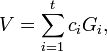
where the  's are a set of coefficients representing a comparison of interest and satisfy
  . The SMCV of contrast variable , denoted by
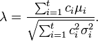
  , is defined as[1]
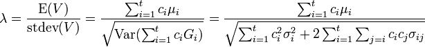
where  is the covariance of
  and
and  . When are independent,
Classifying rule for the strength of group comparisons
The population value (denoted by ) of SMCV can be used to classify the strength of a comparison represented by a contrast variable, as shown in the following table.[1][2]
This classifying rule has a probabilistic basis due to the link between SMCV and c+-probability.[1]
| Effect type | Effect subtype | Thresholds for negative SMCV | Thresholds for positive SMCV |
|---|---|---|---|
| Extra large | Extremely strong |  |  |
| Very strong |  |  | |
| Strong | 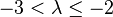 |  | |
| Fairly strong | 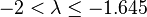 | 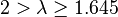 | |
| Large | Moderate |  |  |
| Fairly moderate |  |  | |
| Medium | Fairly weak |  |  |
| Weak |  |  | |
| Very weak |  |  | |
| Small | Extremely weak |  |  |
| No effect |  | ||
Statistical estimation and inference
The estimation and inference of SMCV presented below is for one-factor experiments.[1][2] Estimation and inference of SMCV for multi-factor experiments has also been discussed.[1][3][6]
The estimation of SMCV relies on how samples are obtained in a study. When the groups are correlated, it is usually difficult to estimate the covariance among groups. In such a case, a good strategy is to obtain matched or paired samples (or subjects) and to conduct contrast analysis based on the matched samples. A simple example of matched contrast analysis is the analysis of paired difference of drug effects after and before taking a drug in the same patients. By contrast, another strategy is to not match or pair the samples and to conduct contrast analysis based on the unmatched or unpaired samples. A simple example of unmatched contrast analysis is the comparison of efficacy between a new drug taken by some patients and a standard drug taken by other patients. Methods of estimation for SMCV and c+-probability in matched contrast analysis may differ from those used in unmatched contrast analysis.
Unmatched samples
Consider an independent sample of size  ,
,
from the  group
group  .
.
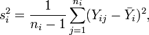
 's are independent. Let
 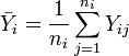 ,
,

and
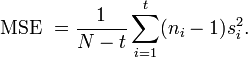
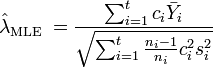
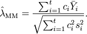
When the  groups have unequal variance, the maximal likelihood estimate (MLE) and method-of-moment estimate (MM) of SMCV () are, respectively[1][2]
and
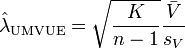
When the groups have equal variance, under normality assumption, the uniformly minimal variance unbiased estimate (UMVUE) of SMCV () is[1][2]
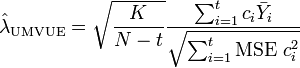
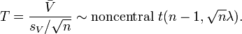
where 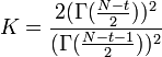 . The confidence interval of SMCV can be made using the following non-central t-distribution:[1][2]
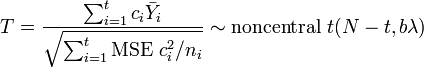
where 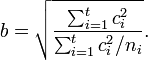
Matched samples
In matched contrast analysis, assume that there are  independent samples
 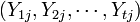 from groups ('s), where
  . Then
the
. Then
the  observed value of a contrast
 is
is 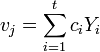 .
Let
.
Let  and
and  be the sample mean and sample variance of the contrast variable , respectively. Under normality assumptions, the UMVUE estimate of SMCV is[1]
where 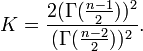
A confidence interval for SMCV can be made using the following non-central t-distribution:[1]
See also
References
- ↑ 1.0 1.1 1.2 1.3 1.4 1.5 1.6 1.7 1.8 1.9 1.10 Zhang XHD (2011). Optimal High-Throughput Screening: Practical Experimental Design and Data Analysis for Genome-scale RNAi Research. Cambridge University Press. ISBN 978-0-521-73444-8.
- ↑ 2.0 2.1 2.2 2.3 2.4 2.5 2.6 Zhang XHD (2009). "A method for effectively comparing gene effects in multiple conditions in RNAi and expression-profiling research". Pharmacogenomics 10: 345–58. doi:10.2217/14622416.10.3.345. PMID 20397965.
- ↑ 3.0 3.1 Zhang XHD (2010). "Assessing the size of gene or RNAi effects in multifactor high-throughput experiments". Pharmacogenomics 11: 199–213. doi:10.2217/PGS.09.136. PMID 20136359.
- ↑ Rosenthal R, Rosnow RL, Rubin DB (2000). Contrasts and Effect Sizes in Behavioral Research. Cambridge University Press. ISBN 0-521-65980-9.
- ↑ Huberty CJ (2002). "A history of effect size indices". Educational and Psychological Measurement 62: 227–40. doi:10.1177/0013164402062002002.
- ↑ 6.0 6.1 Zhang XHD (2010). "Contrast variable potentially providing a consistent interpretation to effect sizes". Journal of Biometrics & Biostatistics 1: 108. doi:10.4172/2155-6180.1000108.
- ↑ Kirk RE (1996). "Practical significance: A concept whose time has come". Educational and Psychological Measurement 56: 746–59. doi:10.1177/0013164496056005002.
- ↑ Cohen J (1962). "The statistical power of abnormal-social psychological research: A review". Journal of Abnormal and Social Psychology 65: 145–53. doi:10.1037/h0045186. PMID 13880271.
- ↑ Glass GV (1976). "Primary, secondary, and meta-analysis of research". Educational Researcher 5: 3–8. doi:10.3102/0013189X005010003.
- ↑ Steiger JH (2004). "Beyond the F test: Effect size confidence intervals and tests of close fit in the analysis of variance and contrast analysis". Psychological Methods 9: 164–82. doi:10.1037/1082-989x.9.2.164.