Standard RAID levels

In computer storage, the standard RAID levels comprise a basic set of RAID configurations that employ the techniques of striping, mirroring, or parity to create large reliable data stores from multiple general-purpose computer hard disk drives (HDDs). The most common types are RAID 0 (striping), RAID 1 and its variants (mirroring), RAID 5 (distributed parity), and RAID 6 (dual parity). RAID levels and their associated data formats are standardized by the Storage Networking Industry Association (SNIA) in the Common RAID Disk Drive Format (DDF) standard.^[1]

RAID 0

Diagram of a RAID 0 setup

RAID 0 (also known as a stripe set or striped volume) splits ("stripes") data evenly across two or more disks, without parity information, redundancy, or fault tolerance. Since RAID 0 provides no fault tolerance or redundancy, the failure of one drive will cause the entire array to fail; as a result of having data striped across all disks, the failure will result in total data loss. This configuration is typically implemented having speed as the intended goal.^[2]^[3] RAID 0 is normally used to increase performance, although it can also be used as a way to create a large logical volume out of two or more physical disks.^[4]

A RAID 0 setup can be created with disks of differing sizes, but the storage space added to the array by each disk is limited to the size of the smallest disk. For example, if a 120 GB disk is striped together with a 320 GB disk, the size of the array will be 240 GB (120 GB × 2).

The diagram shows how the data is distributed into Ax stripes to the disks. Accessing the stripes in the order A1, A2, A3, and so forth provides the illusion of a larger and faster drive. Once the stripe size is defined on creation it needs to be maintained at all times.

Performance

RAID 0 is also used in areas where performance is desired and data integrity is not very important, for example in some computer gaming systems. Although some real-world tests with computer games showed a minimal performance gain when using RAID 0, albeit with some desktop applications benefiting,^[5]^[6] another article examined these claims and concluded: "Striping does not always increase performance (in certain situations it will actually be slower than a non-RAID setup), but in most situations it will yield a significant improvement in performance."^[7]

RAID 1

Diagram of a RAID 1 setup

RAID 1 consists of an exact copy (or mirror) of a set of data on two or more disks; a classic RAID 1 mirrored pair contains two disks. This configuration offers no parity, stripping, or spanning of disk space across multiple disks, since the data is mirrored on all disks belonging to the array, and the array can only be as big as the smallest member disk. This layout is useful when read performance or reliability is more important than write performance or the resulting data storage capacity.^[8]^[9]

The array will continue to operate so long as at least one member drive is operational.^[10]

Performance

Any read request can be serviced and handled by any drive in the array; thus, depending on the nature of I/O load, random read performance of a RAID 1 array may equal up to the sum of each member's performance,^{[lower-alpha 1]} while the write performance remains at the level of a single disk. However, if disks with different speeds are used in a RAID 1 array, overall write performance is equal to the speed of the slowest disk.^[9]^[10]

RAID 2

RAID Level 2

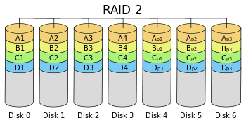
RAID 2 stripes data at the bit (rather than block) level, and uses a Hamming code for error correction. The disks are synchronized by the controller to spin at the same angular orientation (they reach index at the same time), so it generally cannot service multiple requests simultaneously. Extremely high data transfer rates are possible.^[11]^[12]

With all hard disk drives implementing internal error correction, the complexity of an external Hamming code offered little advantage over parity so RAID 2 has been rarely implemented; it is the only original level of RAID that is not currently used.^[11]^[12]

RAID 3

Diagram of a RAID 3 setup of 6-byte blocks and two parity bytes, shown are two blocks of data in different colors.

RAID 3 consists of byte-level striping with a dedicated parity disk. RAID 3 is very rare in practice. One of the characteristics of RAID 3 is that it generally cannot service multiple requests simultaneously. This happens because any single block of data will, by definition, be spread across all members of the set and will reside in the same location. So, any I/O operation requires activity on every disk and usually requires synchronized spindles.

This makes it suitable for applications that demand the highest transfer rates in long sequential reads and writes, for example uncompressed video editing. Applications that make small reads and writes from random disk locations will get the worst performance out of this level.^[12]

The requirement that all disks spin synchronously, a.k.a. lockstep, added design considerations to a level that didn't give significant advantages over other RAID levels, so it quickly became useless and is now obsolete.^[11] Both RAID 3 and RAID 4 were quickly replaced by RAID 5.^[13] RAID 3 was usually implemented in hardware, and the performance issues were addressed by using large disk caches.^[12]

RAID 4

Diagram of a RAID 4 setup with dedicated parity disk with each color representing the group of blocks in the respective parity block (a stripe)

RAID 4, which is rarely used in practice, consists of block-level striping with a dedicated parity disk. As a result of its layout, RAID 4 provides good performance of random reads, while the performance of random writes is low due to the need to write all parity data to a single disk.^[14]

In the example on the right, a read request for block A1 would be serviced by disk 0. A simultaneous read request for block B1 would have to wait, but a read request for B2 could be serviced concurrently by disk 1.

RAID 5

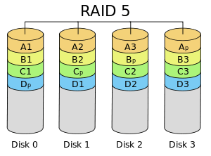
Diagram of a RAID 5 setup with distributed parity with each color representing the group of blocks in the respective parity block (a stripe). This diagram shows left asymmetric algorithm

RAID 5 consists of block-level striping with distributed parity. Unlike in RAID 4, parity information is distributed among the drives. It requires that all drives but one be present to operate. Upon failure of a single drive, subsequent reads can be calculated from the distributed parity such that no data is lost.^[15] RAID 5 requires at least three disks.^[16]

In comparison to RAID 4, RAID 5's distributed parity evens out the stress of a dedicated parity disk among all RAID members. Additionally, read performance is increased since all RAID members participate in serving of the read requests.^[17]

RAID 6

Diagram of a RAID 6 setup, which is identical to RAID 5 other than the addition of a second parity block

RAID 6 extends RAID 5 by adding another parity block; thus, it uses block-level striping with two parity blocks distributed across all member disks.

Performance

RAID 6 does not have a performance penalty for read operations, but it does have a performance penalty on write operations because of the overhead associated with parity calculations. Performance varies greatly depending on how RAID 6 is implemented in the manufacturer's storage architecture—in software, firmware, or by using firmware and specialized ASICs for intensive parity calculations. It can be as fast as a RAID 5 system with one fewer drive (same number of data drives).^[18]

Implementation

According to the Storage Networking Industry Association (SNIA), the definition of RAID 6 is: "Any form of RAID that can continue to execute read and write requests to all of a RAID array's virtual disks in the presence of any two concurrent disk failures. Several methods, including dual check data computations (parity and Reed-Solomon), orthogonal dual parity check data and diagonal parity, have been used to implement RAID Level 6."^[19]

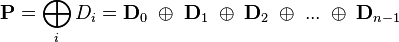
Computing parity

Two different syndromes need to be computed in order to allow the loss of any two drives. One of them, P can be the simple XOR of the data across the stripes, as with RAID 5. A second, independent syndrome is more complicated and requires the assistance of field theory.

To deal with this, the Galois field $GF(m)$ is introduced with $m=2^k$ , where $GF(m) \cong F_2[x]/(p(x))$ for a suitable irreducible polynomial $p(x)$ of degree $k$ . A chunk of data can be written as $d_{k-1}d_{k-2}...d_0$ in base 2 where each $d_i$ is either 0 or 1. This is chosen to correspond with the element $d_{k-1}x^{k-1} + d_{k-2}x^{k-2} + ... + d_1x + d_0$ in the Galois field. Let $D_0,...,D_{n-1} \in GF(m)$ correspond to the stripes of data across hard drives encoded as field elements in this manner (in practice they would probably be broken into byte-sized chunks). If $g$ is some generator of the field and $\oplus$ denotes addition in the field while concatenation denotes multiplication, then $\mathbf{P}$ and $\mathbf{Q}$ may be computed as follows ( $n$ denotes the number of data disks):

\mathbf{P} = \bigoplus_i{D_i} = \mathbf{D}_0 \;\oplus\; \mathbf{D}_1 \;\oplus\; \mathbf{D}_2 \;\oplus\; ... \;\oplus\; \mathbf{D}_{n-1}

\mathbf{Q} = \bigoplus_i{g^iD_i} = g^0\mathbf{D}_0 \;\oplus\; g^1\mathbf{D}_1 \;\oplus\; g^2\mathbf{D}_2 \;\oplus\; ... \;\oplus\; g^{n-1}\mathbf{D}_{n-1}

For a computer scientist, a good way to think about this is that $\oplus$ is a bitwise XOR operator and $g^i$ is the action of a linear feedback shift register on a chunk of data. Thus, in the formula above,^[20] the calculation of P is just the XOR of each stripe. This is because addition in any characteristic two finite field reduces to the XOR operation. The computation of Q is the XOR of a shifted version of each stripe.

Mathematically, the generator is an element of the field such that $g^i$ is different for each nonnegative $i$ satisfying $i < n$ .

If one data drive is lost, the data can be recomputed from P just like with RAID 5. If two data drives are lost or a data drive and the drive containing P are lost, the data can be recovered from P and Q or from just Q, respectively, using a more complex process. Working out the details is extremely hard with field theory. Suppose that $D_i$ and $D_j$ are the lost values with $i \neq j$ . Using the other values of $D$ , constants $A$ and $B$ may be found so that $D_i \oplus D_j = A$ and $g^iD_i \oplus g^jD_j = B$ :

A = \bigoplus_{\ell:\;\ell\not=i\;\mathrm{and}\;\ell\not=j}{D_\ell} = \mathbf{P} \;\oplus\; \mathbf{D}_0 \;\oplus\; \mathbf{D}_1 \;\oplus\; \dots \;\oplus\; \mathbf{D}_{i-1} \;\oplus\; \mathbf{D}_{i+1} \;\oplus\; \dots \;\oplus\; \mathbf{D}_{j-1} \;\oplus\; \mathbf{D}_{j+1} \;\oplus\; \dots \;\oplus\; \mathbf{D}_{n-1}

B = \bigoplus_{\ell:\;\ell\not=i\;\mathrm{and}\;\ell\not=j}{g^{\ell}D_\ell} = \mathbf{Q} \;\oplus\; g^0\mathbf{D}_0 \;\oplus\; g^1\mathbf{D}_1 \;\oplus\; \dots \;\oplus\; g^{i-1}\mathbf{D}_{i-1} \;\oplus\; g^{i+1}\mathbf{D}_{i+1} \;\oplus\; \dots \;\oplus\; g^{j-1}\mathbf{D}_{j-1} \;\oplus\; g^{j+1}\mathbf{D}_{j+1} \;\oplus\; \dots \;\oplus\; g^{n-1}\mathbf{D}_{n-1}

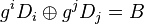Multiplying both sides of the equation for $B$ by $g^{n-i}$ and adding to the former equation yields $(g^{n-i+j}\oplus1)D_j = g^{n-i}B\oplus A$ and thus a solution for $D_j$ , which may be used to compute $D_i$ .

The computation of Q is CPU intensive compared to the simplicity of P. Thus, RAID 6 implemented in software will have a more significant effect on system performance, and a hardware solution will be more complex.

Comparison

The following table provides an overview of some considerations for standard RAID levels. In each case:

Array space efficiency is given as an expression in terms of the number of drives, $n$ ; this expression designates a fractional value between zero and one, representing the fraction of the sum of the drives' capacities that is available for use. For example, if three drives are arranged in RAID 3, this gives an array space efficiency of $1 - 1/n = 1 - 1/3 = 2/3 \approx 67\%$ ; thus, if each drive in this example has a capacity of 250 GB, then the array has a total capacity of 750 GB but the capacity that is usable for data storage is only 500 GB.
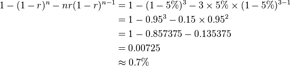
Array failure rate is given as an expression in terms of the number of drives, $n$ , and the drive failure rate, $r$ (which is assumed identical and independent for each drive). For example, if each of three drives has a failure rate of 5% over the next three years, and these drives are arranged in RAID 3, then this gives an array failure rate over the next three years of:

\begin{align} 1 - (1 - r)^{n} - nr(1 - r)^{n - 1} & = 1 - (1 - 5\%)^{3} - 3 \times 5\% \times (1 - 5\%)^{3 - 1} \\ & = 1 - 0.95^{3} - 0.15 \times 0.95^{2} \\ & = 1 - 0.857375 - 0.135375 \\ & = 0.00725 \\ & \approx 0.7\% \end{align}

Level	Description	Minimum number of drives^{[lower-alpha 2]}	Space efficiency	Fault tolerance	Array failure rate^{[lower-alpha 3]}	Read performance	Write performance
RAID 0	Block-level striping without parity or mirroring	2	$1$	None	$1-(1-r)^{n}$	n×	n×
RAID 1	Mirroring without parity or striping	2	$1/n$	n−1 drive failures	$r^{n}$	n×^{[lower-alpha 1]}^[10]	1×^{[lower-alpha 4]}^[10]
RAID 2	Bit-level striping with dedicated Hamming-code parity	3	$1 - 1/n \times \log_2 (n - 1)$	One drive failure^{[lower-alpha 5]}	(Varies)	(Varies)	(Varies)
RAID 3	Byte-level striping with dedicated parity	3	$1 - 1/n$	One drive failure	$1-(1-r)^{n}-nr(1-r)^{n-1}$	(n−1)×	(n−1)×^{[lower-alpha 6]}
RAID 4	Block-level striping with dedicated parity	3	$1 - 1/n$	One drive failure	$1-(1-r)^{n}-nr(1-r)^{n-1}$	(n−1)×	(n−1)×^{[lower-alpha 6]}
RAID 5	Block-level striping with distributed parity	3	$1 - 1/n$	One drive failure	$1-(1-r)^{n}-nr(1-r)^{n-1}$	n×^{[lower-alpha 6]}	(n−1)×^{[lower-alpha 6]}
RAID 6	Block-level striping with double distributed parity	4	$1 - 2/n$	Two drive failures	$1-(1-r)^{n}-nr(1-r)^{n-1}-{n\choose 2}r^{2}(1-r)^{n-2}$	n×^{[lower-alpha 6]}	(n−2)×^{[lower-alpha 6]}

Non-standard RAID levels and non-RAID drive architectures

Main articles: Non-standard RAID levels and Non-RAID drive architectures

Alternatives to the above designs include nested RAID levels, non-standard RAID levels, and non-RAID drive architectures. Non-RAID drive architectures are referred to by similar terms and acronyms, notably JBOD ("just a bunch of disks"), SPAN/BIG, and MAID ("massive array of idle disks").

Notes

↑ 1.0 1.1 Theoretical maximum, as low as single-disk performance in practice.
↑ Assumes a non-degenerate minimum number of drives
↑ Assumes independent, identical rate of failure amongst drives
↑ If disks with different speeds are used in a RAID 1 array, overall write performance is equal to the speed of the slowest disk.
↑ RAID 2 can recover from one drive failure or repair corrupt data or parity when a corrupted bit's corresponding data and parity are good.
↑ 6.0 6.1 6.2 6.3 6.4 6.5 Assumes hardware is fast enough to support

References

↑ "Common raid Disk Data Format (DDF)". SNIA.org. Storage Networking Industry Association. Retrieved 2013-04-23.
↑ "RAID 0 Data Recovery". DataRecovery.net. Retrieved 2015-04-30.
↑ "Understanding RAID". CRU-Inc.com. Retrieved 2015-04-30.
↑ "How to Combine Multiple Hard Drives Into One Volume for Cheap, High-Capacity Storage". LifeHacker.com. 2013-02-26. Retrieved 2015-04-30.
↑ "Western Digital's Raptors in RAID-0: Are two drives better than one?". AnandTech.com. AnandTech. July 1, 2004. Retrieved 2007-11-24.
↑ "Hitachi Deskstar 7K1000: Two Terabyte RAID Redux". AnandTech.com. AnandTech. April 23, 2007. Retrieved 2007-11-24.
↑ "RAID 0: Hype or blessing?". Tweakers.net. Tweakers.net. August 7, 2004. Retrieved 2008-07-23.
↑ "FreeBSD Handbook: 19.3. RAID 1 – Mirroring". FreeBSD.org. 2014-03-23. Retrieved 2014-06-11.
↑ 9.0 9.1 "Which RAID Level is Right for Me?: RAID 1 (Mirroring)". Adaptec.com. Adaptec. Retrieved 2014-01-02.
↑ 10.0 10.1 10.2 10.3 "Selecting the Best RAID Level: RAID 1 Arrays (Sun StorageTek SAS RAID HBA Installation Guide)". Docs.Oracle.com. Oracle Corporation. 2010-12-23. Retrieved 2014-01-02.
↑ 11.0 11.1 11.2 Derek Vadala (2003). Managing RAID on Linux. O'Reilly Series (illustrated ed.). O'Reilly. p. 6. ISBN 9781565927308.
↑ 12.0 12.1 12.2 12.3 Evan Marcus, Hal Stern (2003). Blueprints for high availability (2, illustrated ed.). John Wiley and Sons. p. 167. ISBN 9780471430261.
↑ Michael Meyers, Scott Jernigan (2003). Mike Meyers' A+ Guide to Managing and Troubleshooting PCs (illustrated ed.). McGraw-Hill Professional. p. 321. ISBN 9780072231465.
↑ Ramesh Natarajan (2011-11-21). "RAID 2, RAID 3, RAID 4 and RAID 6 Explained with Diagrams". TheGeekStuff.com. Retrieved 2015-01-02.
↑ Chen, Peter; Lee, Edward; Gibson, Garth; Katz, Randy; Patterson, David (1994). "RAID: High-Performance, Reliable Secondary Storage". ACM Computing Surveys 26: 145–185. doi:10.1145/176979.176981.
↑ "RAID 5 Data Recovery FAQ". VantageTech.com. Vantage Technologies. Retrieved 2014-07-16.
↑ Koren, Israel. "Basic RAID Organizations". ECS.UMass.edu. UMass Dept. of Electrical and Computer Engineering. Retrieved 2014-11-04.
↑ Rickard E. Faith (13 May 2009). "A Comparison of Software RAID Types".
↑ "Dictionary R". SNIA.org. Storage Networking Industry Association. Retrieved 2007-11-24.
↑ Anvin, H. Peter (May 21, 2009). "The Mathematics of RAID-6" (PDF). Kernel.org. Linux Kernel Organization. Retrieved November 4, 2009.

External links

Animations and details on RAID levels 0, 1, and 5, Dell (archived from the original on February 20, 2009)
IBM summary on RAID levels
RAID 5 parity explanation and checking tool
RAID Calculator for Standard RAID Levels and Other RAID Tools
Redundant Arrays of Inexpensive Disks (RAIDs), Chapter 38 from the Operating Systems: Three Easy Pieces book
Sun StorEdge 3000 Family Configuration Service 2.5 User’s Guide: RAID Basics