Stable distribution
|
Probability density function
| |
|
Cumulative distribution function
| |
| Parameters |
α ∈ (0, 2] — stability parameter |
|---|---|
| Support | x ∈ R, or x ∈ [μ, +∞) if α < 1 and β = 1, or x ∈ (-∞, μ] if α < 1 and β = −1 |
| not analytically expressible, except for some parameter values | |
| CDF | not analytically expressible, except for certain parameter values |
| Mean | μ when α > 1, otherwise undefined |
| Median | μ when β = 0, otherwise not analytically expressible |
| Mode | μ when β = 0, otherwise not analytically expressible |
| Variance | 2c2 when α = 2, otherwise infinite |
| Skewness | 0 when α = 2, otherwise undefined |
| Ex. kurtosis | 0 when α = 2, otherwise undefined |
| Entropy | not analytically expressible, except for certain parameter values |
| MGF | undefined |
| CF |
 |


![\exp\!\Big[\; it\mu - |c\,t|^\alpha\,(1-i \beta\,\mbox{sgn}(t)\Phi) \;\Big],](../I/m/a3ff334ccf052804905cfb91f4fa1a6e.png)
In probability theory, a distribution is said to be stable (or a random variable is said to be stable) if a linear combination of two independent copies of a random sample has the same distribution, up to location and scale parameters. The stable distribution family is also sometimes referred to as the Lévy alpha-stable distribution, after Paul Lévy, the first mathematician to have studied it.[1][2]
The importance of stable probability distributions is that they are "attractors" for properly normed sums of independent and identically-distributed (iid) random variables. The normal distribution defines a family of stable distributions. By the classical central limit theorem the properly normed sum of a set of random variables, each with finite variance, will tend towards a normal distribution as the number of variables increases. Without the finite variance assumption the limit may be a stable distribution. Mandelbrot referred to stable distributions that are non-normal as "stable Paretian distributions",[3][4][5] after Vilfredo Pareto. Mandelbrot referred to "positive" stable distributions (meaning maximally skewed in the positive direction) with 1<α<2 as "Pareto-Levy distributions".[1]
q-analogs of all symmetric stable distributions have been defined, and these recover the usual symmetric stable distributions in the limit of q → 1.[6]
Definition
A non-degenerate distribution is a stable distribution if it satisfies the following property:
- Let X1 and X2 be independent copies of a random variable X. Then X is said to be stable if for any constants a > 0 and b > 0 the random variable aX1 + bX2 has the same distribution as cX + d for some constants c > 0 and d. The distribution is said to be strictly stable if this holds with d = 0.[7]
Since the normal distribution, the Cauchy distribution, and the Lévy distribution all have the above property, it follows that they are special cases of stable distributions.
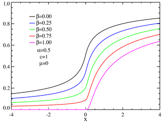
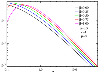
Such distributions form a four-parameter family of continuous probability distributions parametrized by location and scale parameters μ and c, respectively, and two shape parameters β and α, roughly corresponding to measures of asymmetry and concentration, respectively (see the figures).
Although the probability density function for a general stable distribution cannot be written analytically, the general characteristic function can be. Any probability distribution is given by the Fourier transform of its characteristic function φ(t) by:
A random variable X is called stable if its characteristic function can be written as[7][8]
![\varphi(t;\alpha,\beta,c,\mu) = \exp\left[~it\mu\!-\!|c t|^\alpha\,(1\!-\!i \beta\,\textrm{sgn}(t)\Phi)~\right]](../I/m/125baaf6283c0ab1f51209bd9b3e700d.png)
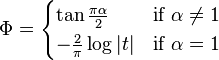
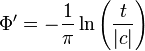
where sgn(t) is just the sign of t and Φ is given by
for all α except α = 1 in which case:

μ ∈ R is a shift parameter, β ∈ [−1, 1], called the skewness parameter, is a measure of asymmetry. Notice that in this context the usual skewness is not well defined, as for α < 2 the distribution does not admit 2nd or higher moments, and the usual skewness definition is the 3rd central moment.
In the simplest case β = 0, the characteristic function is just a stretched exponential function; the distribution is symmetric about μ and is referred to as a (Lévy) symmetric alpha-stable distribution, often abbreviated SαS.
When α < 1 and β = 1, the distribution is supported by [μ, ∞).
The parameter |c| > 0 is a scale factor which is a measure of the width of the distribution and α is the exponent or index of the distribution and specifies the asymptotic behavior of the distribution for α < 2.
Parameterizations
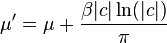
The above definition is only one of the parameterizations in use for stable distributions; it is the most common but is not continuous in the parameters. For example, for the case α = 1 we could replace Φ by:[7]
and μ by
This parameterization has the advantage that we may define a standard distribution using

and

The pdf for all α will then have the following standardization property:

The distribution
A stable distribution is therefore specified by the above four parameters. It can be shown that any non-degenerate stable distribution has a smooth (infinitely differentiable) density function.[9] If  denotes the density of X and Y is the sum of independent copies of X:
then Y has the density  with
with
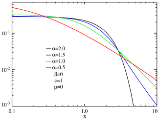
The asymptotic behavior is described, for α< 2, by:[10]

where Γ is the Gamma function (except that when α < 1 and β = ±1, the tail vanishes to the left or right, resp., of μ). This "heavy tail" behavior causes the variance of stable distributions to be infinite for all α < 2. This property is illustrated in the log-log plots below.
When α = 2, the distribution is Gaussian (see below), with tails asymptotic to exp(−x2/4c2)/(2c√π).
Properties
- All stable distributions are infinitely divisible.
- With the exception of the normal distribution (α = 2), stable distributions are leptokurtotic and heavy-tailed distributions.
- Closure under convolution
Stable distributions are closed under convolution for a fixed value of α. Since convolution is equivalent to multiplication of the Fourier-transformed function, it follows that the product of two stable characteristic functions with the same α will yield another such characteristic function. The product of two stable characteristic functions is given by:
![\exp\left[it\mu_1+it\mu_2 - |c_1 t|^\alpha - |c_2 t|^\alpha +i\beta_1|c_1 t|^\alpha\textrm{sgn}(t)\Phi +i\beta_2|c_2 t|^\alpha\,\textrm{sgn}(t)\Phi \right]](../I/m/b8ae6ebfe5336a336bfe99e32fc0b744.png)
Since Φ is not a function of the μ, c or β variables it follows that these parameters for the convolved function are given by:
In each case, it can be shown that the resulting parameters lie within the required intervals for a stable distribution.
A generalized central limit theorem
Another important property of stable distributions is the role that they play in a generalized central limit theorem. The central limit theorem states that the sum of a number of independent and identically distributed (i.i.d.) random variables with finite variances will tend to a normal distribution as the number of variables grows.
A generalization due to Gnedenko and Kolmogorov states that the sum of a number of random variables with a power-law tail (Paretian tail) distributions decreasing as |x|−α−1 where 0 < α < 2 (and therefore having infinite variance) will tend to a stable distribution  as the number of summands grows.[8][11] If α>2 then the sum converges to a stable distribution with stability parameter equal to 2, i.e. a Gaussian distribution.[12]
Special cases
There is no general analytic solution for the form of p(x). There are, however three special cases which can be expressed in terms of elementary functions as can be seen by inspection of the characteristic function.
- For α = 2 the distribution reduces to a Gaussian distribution with variance σ2 = 2c2 and mean μ; the skewness parameter β has no effect.[7][8]
- For α = 1 and β = 0 the distribution reduces to a Cauchy distribution with scale parameter c and shift parameter μ.[7][8]
- For α =1/2 and β = 1 the distribution reduces to a Lévy distribution with scale parameter c and shift parameter μ.[7][13]
Note that the above three distributions are also connected, in the following way: A standard Cauchy random variable can be viewed as a mixture of Gaussian random variables (all with mean zero), with the variance being drawn from a standard Lévy distribution. And in fact this is a special case of a more general theorem [14] which allows any symmetric alpha-stable distribution to be viewed in this way (with the alpha parameter of the mixture distribution equal to twice the alpha parameter of the mixing distribution—and the beta parameter of the mixing distribution always equal to one).
A general closed form expression for stable PDF's with rational values of α is available in terms of Meijer G-functions.[15] Fox H-Functions can also be used to express the stable probability density functions. For simple rational numbers, the closed form expression is often in terms of less complicated special functions. Several closed form expressions having rather simple expressions in terms of special functions are available.[14] In the table below, PDF's expressible by elementary functions are indicated by an E and those that are expressible by special functions are indicated by an s.[14]
| α | |||||||
|---|---|---|---|---|---|---|---|
| 1/3 | 1/2 | 2/3 | 1 | 4/3 | 3/2 | 2 | |
| β=0 | s | s | s | E | s | s | E |
| β=1 | s | E | s | s | s | ||
Some of the special cases are known by particular names:
- For α = 1 and β = 1, the distribution is a Landau distribution which has a specific usage in physics under this name.
- For α = 3/2 and β = 0 the distribution reduces to a Holtsmark distribution with scale parameter c and shift parameter μ.[14]
Also, in the limit as c approaches zero or as α approaches zero the distribution will approach a Dirac delta function δ(x−μ).
Series representation
The stable distribution can be restated as the real part of a simpler integral:[13]
![f(x;\alpha,\beta,c,\mu)=\frac{1}{\pi}\Re\left[ \int_0^\infty e^{it(x-\mu)}e^{-(ct)^\alpha(1-i\beta\Phi)}\,dt\right].](../I/m/69957390774fb78133302bc9affbd88e.png)
Expressing the second exponential as a Taylor series, we have:
![f(x;\alpha,\beta,c,\mu)=\frac{1}{\pi}\Re\left[ \int_0^\infty e^{it(x-\mu)}\sum_{n=0}^\infty\frac{(-qt^\alpha)^n}{n!}\,dt\right]](../I/m/44b919211409d6d66d2279ec4b67eb9e.png)
where  . Reversing the order of integration and summation, and carrying out the integration yields:
![f(x;\alpha,\beta,c,\mu)=\frac{1}{\pi}\Re\left[ \sum_{n=1}^\infty\frac{(-q)^n}{n!}\left(\frac{i}{x-\mu}\right)^{\alpha n+1}\Gamma(\alpha n+1)\right]](../I/m/0caaa5dfba5511c1df778311e55f898b.png)
which will be valid for x ≠ μ and will converge for appropriate values of the parameters. (Note that the n = 0 term which yields a delta function in x−μ has therefore been dropped.) Expressing the first exponential as a series will yield another series in positive powers of x−μ which is generally less useful.
Applications
Stable distributions owe their importance in both theory and practice to the generalization of the central limit theorem to random variables without second (and possibly first) order moments and the accompanying self-similarity of the stable family. It was the seeming departure from normality along with the demand for a self-similar model for financial data (i.e. the shape of the distribution for yearly asset price changes should resemble that of the constituent daily or monthly price changes) that led Benoît Mandelbrot to propose that cotton prices follow an alpha-stable distribution with α equal to 1.7.[16] Lévy distributions are frequently found in analysis of critical behavior and financial data.[8]
They are also found in spectroscopy as a general expression for a quasistatically pressure broadened spectral line.[13]
Lévy distribution of solar flare waiting time events (time between flare events) was demonstrated for CGRO BATSE hard x-ray solar flares December 2001. Analysis of the Lévy statistical signature revealed that two different memory signatures were evident; one related to the solar cycle and the second whose origin appears to be associated with a localized or combination of localized solar active region effects.[17]
See also
- Lévy flight
- Lévy process
- Fractional quantum mechanics
- Other "power law" distributions
- Stable and tempered stable distributions with volatility clustering – financial applications
- Multivariate stable distribution
- Discrete-stable distribution
Notes
- ↑ 1.0 1.1 B. Mandelbrot, The Pareto-Lévy Law and the Distribution of Income, International Economic Review 1960 http://www.jstor.org/stable/2525289
- ↑ Paul Lévy, Calcul des probabilités 1925
- ↑ B.Mandelbrot, Stable Paretian Random Functions and the Multiplicative Variation of Income, Econometrica 1961 http://www.jstor.org/stable/pdfplus/1911802.pdf
- ↑ B. Mandelbrot, The variation of certain Speculative Prices, The Journal of Business 1963
- ↑ Eugene F. Fama, Mandelbrot and the Stable Paretian Hypothesis, The Journal of Business 1963
- ↑ Umarov, Sabir; Tsallis, Constantino, Gell-Mann, Murray and Steinberg, Stanly (2010). "Generalization of symmetric α-stable Lévy distributions for q>1". J Math Phys. (American Institute of Physics) 51 (3). arXiv:0911.2009. Bibcode:2010JMP....51c3502U. doi:10.1063/1.3305292. PMC 2869267. PMID 20596232. Retrieved 2011-07-29.
- ↑ 7.0 7.1 7.2 7.3 7.4 7.5 Nolan (2009)
- ↑ 8.0 8.1 8.2 8.3 8.4 Voit, Johannes (2003). The Statistical Mechanics of Financial Markets (Texts and Monographs in Physics). Springer-Verlag. ISBN 3-540-00978-7. (Section 5.4.3) http://books.google.it/books?id=6zUlh_TkWSwC&dq=The+Statistical+Mechanics+of+Financial+Markets&hl=it&source=gbs_navlinks_s
- ↑ Nolan (2009; Theorem 1.9)
- ↑ Nolan (2009; Theorem 1.12)
- ↑ B.V. Gnedenko, A.N. Kolmogorov. Limit distributions for sums of independent random variables, Cambridge, Addison-Wesley 1954 http://books.google.it/books/about/Limit_distributions_for_sums_of_independ.html?id=rYsZAQAAIAAuJ&redir_esc=y
- ↑ Vladimir V. Uchaikin, Vladimir M. Zolotarev, Chance and Stability: Stable Distributions and their Applications, De Gruyter 1999 http://books.google.it/books/about/Chance_and_Stability.html?id=Y0xiwAmkb_oC&redir_esc=y
- ↑ 13.0 13.1 13.2 Peach, G. (1981). "Theory of the pressure broadening and shift of spectral lines". Advances in Physics 30 (3): 367–474. Bibcode:1981AdPhy..30..367P. doi:10.1080/00018738100101467. (Section 4.5)
- ↑ 14.0 14.1 14.2 14.3 Lee, W.H. (2010). Continuous and discrete properties of stochastic processes (PhD thesis). The University of Nottingham.
- ↑ Zolotarev, V.M. (1995). "On Representation of Densities of Stable Laws by Special Functions". Theory Probab. Appl. (SIAM) 39 (2): 354–362. doi:10.1137/1139025. Retrieved 2011-08-15.
- ↑ Mandelbrot, B., New methods in statistical economics The Journal of Political Economy, 71 #5, 421-440 (1963).
- ↑ Leddon, D., A statistical Study of Hard X-Ray Solar Flares
References
- Nolan, John P. (2009). "Stable Distributions: Models for Heavy Tailed Data" (PDF). Retrieved 2009-02-21.
Further reading
- Feller, W. (1971) An Introduction to Probability Theory and Its Applications, Volume 2. Wiley. ISBN 0-471-25709-5
- Gnedenko, B. V.; Kolmogorov, A. N. (1954). Limit Distributions for Sums of Independent Random Variables. Addison-Wesley.
- Ibragimov, I.; Linnik, Yu (1971). Independent and Stationary Sequences of Random Variables. Wolters-Noordhoff Publishing Groningen, The Netherlands.
- Matsui, M.; Takemura, A. (2004). "Some improvements in numerical evaluation of symmetric stable density and its derivatives" (PDF). CIRGE Discussion paper. Retrieved April 19, 2013.
- Rachev, S.; Mittnik, S. (2000). "Stable Paretian Models in Finance". Wiley. ISBN 978-0-471-95314-2.
- Samorodnitsky, G.; Taqqu, M. (1994). "Stable Non-Gaussian Random Processes: Stochastic Models with Infinite Variance (Stochastic Modeling Series)". Chapman and Hall/CRC. ISBN 978-0-412-05171-5.
- Zolotarev, V.M. (1986). One-dimensional Stable Distributions. American Mathematical Society. ISBN 0821898159.
- Martin, Doug; Rachev, Zari; Siboulet, Frederic (2003). "Phi-alpha optimal portfolios and extreme risk management". The Best of Wilmott 1, Wiley, 2004. ISBN 978-0-470-02351-8.
External links
- PlanetMath stable random variable article
- John P. Nolan page on stable distributions
- Applications of stable laws in finance.