Squirmer

Shaker, $\beta=-\infty$	Pusher, $\beta=-5$	Neutral, $\beta=0$	Puller, $\beta=5$	Shaker, $\beta=\infty$	Passive particle
Shaker, $\beta=-\infty$	Pusher, $\beta=-5$	Neutral, $\beta=0$	Puller, $\beta=5$	Shaker, $\beta=\infty$	Passive particle
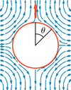
Velocity field of squirmer and passive particle (top row: lab frame, bottom row: swimmer frame)

The squirmer is a model for a spherical microswimmer swimming in Stokes flow. The squirmer model has been introduced by James Lighthill in 1952 and refined and used to model Paramecium by John Blake in 1971.^[1] ^[2] Blake used the squirmer model to describe the flow generated by a carpet of beating short filaments called cilia on the surface of Paramecium. Today, the squirmer is a standard model for the study of self-propelled particles, such as Janus particles, in Stokes flow.^[3]

Velocity field in particle frame

Here we give the flow field of a squirmer in the case of a non-deformable axisymmetric spherical squirmer (radius $R$ ).^[1]^[2] These expressions are given in a spherical coordinate system.

$u_r(r,\theta)=\frac 2 3 \left(\frac{R^3}{r^3} -1\right)B_1P_1(\cos\theta)+\sum_{n=2}^{\infty}\left(\frac{R^{n+2}}{r^{n+2}}-\frac{R^n}{r^n}\right)B_nP_n(\cos\theta)\;,$
$u_{\theta}(r,\theta)=\frac 2 3 \left(\frac{R^3}{2r^3}+1\right)B_1V_1(\cos\theta)+\sum_{n=2}^{\infty}\frac 1 2\left(n\frac{R^{n+2}}{r^{n+2}}+(2-n)\frac{R^n}{r^n}\right)B_nV_n(\cos\theta)\;.$

Here $B_n$ are constant coefficients, $P_n(\cos\theta)$ are Legendre polynomials, and $V_n(\cos\theta)=\frac{-2}{n(n+1)}\partial_{\theta}P_n(\cos\theta)$ .
One finds $P_1(\cos\theta)=\cos\theta, P_2(\cos\theta)=\tfrac 1 2 (3\cos^2\theta-1), \dots, V_1(\cos\theta)=\sin\theta, V_2(\cos\theta)= \tfrac{1}{2} \sin 2\theta, \dots$ .
The expressions above are in the frame of the moving particle. At the interface one finds $u_{\theta}(R,\theta)=\sum_{n=1}^{\infty} B_nV_n$ and $u_r(R,\theta)=0$ .

Swimming speed and lab frame

By using the Lorentz Reciprocal Theorem, one finds the velocity vector of the particle 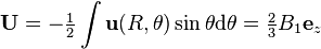$\mathbf{U}=-\tfrac{1}{2} \int \mathbf{u}(R,\theta)\sin\theta\mathrm{d}\theta=\tfrac 2 3 B_1 \mathbf{e}_z$ . The flow in a fixed lab frame is given by $\mathbf{u}^L=\mathbf{u}+\mathbf{U}$ :

$u_r^L(r,\theta)=\frac{R^3}{r^3}UP_1(\cos\theta)+\sum_{n=2}^{\infty}\left(\frac{R^{n+2}}{r^{n+2}}-\frac{R^n}{r^n}\right)B_nP_n(\cos\theta)\;,$
$u_{\theta}^L(r,\theta)=\frac{R^3}{2r^3}UV_1(\cos\theta)+\sum_{n=2}^{\infty}\frac 1 2\left(n\frac{R^{n+2}}{r^{n+2}}+(2-n)\frac{R^n}{r^n}\right)B_nV_n(\cos\theta)\;.$

with swimming speed $U=|\mathbf{U}|$ . Note, that $\lim_{r\rightarrow\infty}\mathbf{u}^L=0$ and $u^L_r(R,\theta)\neq 0$ .

Structure of the flow and squirmer parameter

The series above are often truncated at $n=2$ in the study of far field flow, $r\gg R$ . Within that approximation, $u_{\theta}(R,\theta)=B_1\sin\theta+\tfrac 1 2 B_2 \sin 2 \theta$ , with squirmer parameter 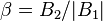$\beta=B_2/|B_1|$ . The first mode $n=1$ characterizes a hydrodynamic stokeslet with decay $\propto 1/r^3$ (and with that the swimming speed $U$ ). The second mode $n=2$ corresponds to a hydrodynamic stresslet or force dipole with decay $\propto 1/r^2$ .^[4] Thus, $\beta$ gives the ratio of both contributions and the direction of the force dipole. $\beta$ is used to categorize microswimmers into pushers, pullers and neutral swimmers.^[5]

Swimmer Type	pusher	neutral swimmer	puller	shaker	passive particle
Squirmer Parameter	$\beta<0$	$\beta=0$	$\beta>0$	$\beta=\pm\infty$
Decay of Velocity Far Field	$\mathbf{u}\propto 1/r^2$	$\mathbf{u}\propto 1/r^3$	$\mathbf{u}\propto 1/r^2$	$\mathbf{u}\propto 1/r^2$	$\mathbf{u}\propto 1/r$
Biological Example	E.Coli	Paramecium	Chlamydomonas reinhardtii

As can be seen in the figures above, the (lab frame) velocity field of the passive particle corresponds to a monopole. Furthermore, the $B_1$ mode corresponds to a dipole (see case $\beta=0$ ) and the $B_2$ mode corresponds to a quadrupole (see cases $\beta\neq0$ ).

References

↑ 1.0 1.1 Lighthill, M. J. (1952). "On the squirming motion of nearly spherical deformable bodies through liquids at very small reynolds numbers". Communications on Pure and Applied Mathematics 5 (2): 109–118. doi:10.1002/cpa.3160050201. ISSN 0010-3640.
↑ 2.0 2.1 Blake, J. R. (1971). "A spherical envelope approach to ciliary propulsion". Journal of Fluid Mechanics 46 (01): 199. doi:10.1017/S002211207100048X. ISSN 0022-1120.
↑ Bickel, Thomas; Majee, Arghya; Würger, Alois (2013). "Flow pattern in the vicinity of self-propelling hot Janus particles". Physical Review E 88 (1). doi:10.1103/PhysRevE.88.012301. ISSN 1539-3755.
↑ Happel, John; Brenner, Howard (1981). "Low Reynolds number hydrodynamics". doi:10.1007/978-94-009-8352-6. ISSN 0921-3805.
↑ Downton, Matthew T; Stark, Holger (2009). "Simulation of a model microswimmer". Journal of Physics: Condensed Matter 21 (20): 204101. doi:10.1088/0953-8984/21/20/204101. ISSN 0953-8984.